Ah, the red-tinged realm of the rubber ducky comes to an end.
The Ayn Gang returned to The Hillfrom its recent long search for The Lost Stones of Gonad.
That search came on the 'heals' of their ritual bath following their shenanigans in the Feast of Ayn (which they had confused with a midterm election) (Ayn Rand: Patron Saint of The Plutocracy, 2, 3, 4).
Because the Feast of Ayn (Ayn is Russian) is another Russian thingy (which among other thingys seeks to eradicate the common good), they sought to sing away their confusion using the lyrics to "Alt-Lang-Sigh-On".
At the other end of confusion avenue, the Senate engineered a cathartic dynamic just as The Cathartic Feast festivities were getting under way.
Yes, the Senate did a very rare thingy, especially in these days daze.
In as much as The Cathartic Feast follows the Feast of Ayn and the rubber ducky bath, they tried not to jump the shark:
"The Senate unanimously approved the legislation Wednesday night to keep the government funded through Feb. 8."
(CNBC). "Those who stayed" (TWS) did not take the bath nor join the search for The Lost Stones of Gonad.
So ... they did a mind meld instead, which resulted in a unanimous thingy (a thingy required by the Tenets of Catharsis).
"Not to worry," TWS reminded the newbies, because The Cathartic Feast gives rise to one of the spiritual joys of Congress.
"Have we forgotten the congressional veto override?" TWS asked.
The tenets of the Cathartic Feast require a unanimous Senate vote (at the beginning of the feast), which must be followed by a preznidential veto (which can only take place when there is a clueless preznit in the Whut? House).
Preznit Yellow One The Last has promised a veto, so let the Cathartic Feast begin!
III. Nancy The Last
When Boy "Ayn" Ryan hands the now-tear-stained gavel to Nancy The Last, she will fulfill her vow to quickly send a clean bill of goods (BOG) over to TWS.
Because it will be as exemplary as the BOG that was unanimously voted for in the Old Senate, which Yellow One The Last vetoed, this BOG is the finger food for The Cathartic Feast (some call it the food of the BOGs).
IV. Conclusion
The Shape Shifters of Bullshitistan were not pleased with all the catharsis taking place, mainly because it promotes honesty, truth, and facts (The Shapeshifters of Bullshitistan, 2, 3, 4, 5, 6, 7, 8, 9, 10, 11, 12, 13, 14, 15, 16).
That in itself could be a death knell to The New World Odor, so they have vowed not to change their diapers for as long as Yellow One The Last whines about his yellow Awe Topsy tweet.
According to my research, these yellow rubber ducky countries block Dredd Blog: Cuba, Fiji, India, Iran, Kazakhstan, Kyrgyzstan, Pakistan, People's Republic of China, Russian Federation, Syrian Arab Republic, Turkey, Vietnam, Yemen, and of course Bullshitistan.
The next post in this series is here, the previous post in this series is here.
In this series I have written about the difficulty of calculating plume volume:
"Thus, at this time I am not able to report on any specific tidewater glacier's plume width or, therefore, any specific glacier's plume volume.
At this point I am left with the meta-level computations which I am blogging about at this time." - The Ghost Plumes - 2 ...
"That melting of the tidewater glaciers is taking place is not debatable, however, the amount of melt water in hypothetical thermodynamic plumes ... is quite debatable since the concept is "embryonic" at this point ... The object of the use of that paper's ["by R. Bindschadler et al."] conclusions is to determine a ball-park figure for thermodynamic plume flow volume along the world's longest wall of ice ..." - The Ghost Plumes - 4
(etc., etc.). The experimental numbers I have calculated by using the data of that paper were way too high, so I changed them (explained below).
Assuming the data and calculations in that paper ["by R. Bindschadler et al."] are correct in substantial degree, I changed plume flow timespan.
NOTE that the Appendices (A, B, C, D, E, and F) now contain values required to raise sea level by 1 mm in each Area and each zone within each Area.
Those figures are quite accurate and show that this could be a significant undertaking.
This approach also explains why I am interested in being able to calculate the actual ghost plume melt water volume with the best precision we can derive.
But, until I can find the sea level and changes in it caused by tides around Antarctica, I can't calculate the vertical distance from the grounding line to the mean sea level, i.e. the middle level between high and low tides.
I need that to zero in on actual plume flow volume.
II. Focus
The current idealized plume height value (pH) is obviously not the real world value because not all grounding lines are at the same depth.
Even glaciers that are next to each other can have significantly different grounding line depths (A Tale of Two Glaciers).
Furthermore, the fact that the plume height (pH) varies from year to year in the Appendices is due to at least two factors:
1) that value is calculated from in situ measurements taken in a zone at different times, in different years, at different depths, by different research crews, in different ice, weather, and ocean conditions,
2) those in situ values are only used if the TEOS-10 toolkit indicates (using "CT", "SA", and "P" values calculated from the in situ measurements) that an ice face section will be melted by those conditions.
Thus, this is a beginning point like "A New Mersenne Prime Discovery" which will be honed by a search for the missing depth and width measurements of Antarctic tidewater glaciers (confirmed search clues gladly accepted).
The pH variation can be zeroed in on a bit better by the new Appendices values (A, B, C, D, E, and F) based on a 1 mm sea level rise.
Plume flow changes are influenced by the flow of the substantial current that reaches completely around Antarctica (Mysterious Zones of Antarctica - 3).
They will not be able to be accurately ascertained until the distance between the grounding line and the ocean surface is known more accurately.
And don't forget pH (plume height) is not the same as glacier ice face height.
The variable pH is only the span of melt that generates a plume.
If calving, thermal plumes (ghost plumes), and basal melt plumes can make up the difference, that will balance the sea level change "budget" which is about 3.4 mm per year (global mean average) at this time.
IV. New Developments
Since acquiring the Bindschadler database and starting this new approach, I can see that the research is worthwhile.
The next post in this series is here, the previous post in this series is here.
There was a conversation between a lawman and a lawless man.
It went something like this: "Why do you rob banks?" asked the lawman, to which the lawless man replied "That is where the money is!"
Readers of Dredd Blog may wonder why I care about a minority class of glaciers (tidewater glaciers) and a minor section of those glaciers (their terminus) which are found in tidewaters along the coasts of Greenland and Antarctica (e.g. The Ghost Plumes, 2, 3, 4; In Pursuit of Plume Theory, 2, 3).
The answer to that wonder is illustrated in Fig. 1, which shows two glaciers in Greenland.
One of those glaciers is melting rapidly, the other one which is next to it, is melting very slowly by comparison.
II. What Is And What Is Not Questioned
The melt-rate difference between the two side-by-side glaciers is not questioned:
"Tracy and Heilprin, marine-terminating glaciers that drain into the eastern end of Inglefield Gulf in northwest Greenland, exhibit remarkably different behaviors despite being adjacent systems. Losing mass since 1892, Tracy Glacier has dramatically accelerated, thinned, and retreated. Heilprin has retreated only slightly during the last century and has remained almost stationary in the most recent decade. Previous studies suggest that Tracy’s base is deeper than Heilprin’s at the calving front (over 600 m, as opposed to the 350 m depth at Heilprin), which exposes it to warmer subsurface waters, resulting in more rapid retreat. We investigate the local oceanographic conditions in Inglefield Gulf and their interactions with Tracy and Heilprin using data collected in 2016 and 2017 as part of NASA’s Oceans Melting Greenland mission. Based on improved estimates of the fjord geometry and 20 temperature and salinity profiles near the fronts of these two glaciers, we find clear evidence that fjord waters are modified by ocean-ice interactions with Tracy Glacier. We find that Tracy thinned by 9.9 m near its terminus between 2016 and 2017, while Heilprin thinned by only 1.8 m."
(Willis et al. 2018, Oceanography, Volume 31, No. 2, emphasis added). But the explanation for the contrast in melt-rate between the two glaciers is questioned.
The authors of that paper adopt basal melt plume theory (BPT) to try to explain the phenomenon.
They do so even when the basal melt water volume of Heilprin is much larger than that of Tracy:
"Heilprin Glacier has a much larger runoff catchment [than Tracy], resulting in higher peak subglacial discharge [but less ice melt and grounding line retreat]"
(ibid). Furthermore, the BPT theory is not robust.
Nevertheless, it is currently in practically universal use when researchers try to explain tidewater basal glacial melt.
Using BPT alone, they are evidently unaware of the hypothesis of thermodynamic forcing (ghost plumes).
They also resort to BPT even though the following statement is found in the literature:
"However, without direct observations of subglacial channels/outlets or their upwelling plumes, the geometries used in these [BPT] plume models are unvalidated ... Although [BPT] plume theory is idealized, it is currently the primary (almost exclusive) tool for tuning or parameterizing plumes in numerical models."
(Surveying subglacial discharge plumes, emphasis added). There is no consideration that I am aware of for the thermodynamic forces I have set forth in previous Dredd Blog posts outlining the hypothesis of the ghost plumes, or Ghost Plume Theory (GPT).
III. Look For The Ocean Heat
The essence of general "ocean heat" or specific "tidewater heat" and its impact on tidewater glaciers is not properly addressed by analyzing atmospheric-temperature-caused glacial surface melt, mixed with basal friction melt, as is typically done in current research papers (In Pursuit of Plume Theory, 2, 3; The Ghost Plumes, 2, 3, 4).
Those basal melt dynamics produce fresh basal melt water that exits at the glacier's grounding line, but IMO that is not sufficient to explain the contrast between Tracy and Heilprin.
When we search for "ocean heat" the place to look and analyze is ocean water instead of basal melt water (In Search Of Ocean Heat, 2, 3).
The specific quantity of potential enthalpy to look for in seawater that comes in contact with tidewater glaciers is the amount of potential enthalpy required to melt the glacial ice.
The authors of that paper stated that "[t]he grounded ice boundary is 53 610 km long; 74 % abuts to floating ice shelves or outlet glaciers, 19 % is adjacent to open or sea-ice covered ocean, and 7 % of the boundary ice terminates on land" (ibid, Abstract).
The 74% of "53,610 km long" and "27,521 km and is discontinuous" are figures in the paper that I want to focus on in this post (among other things).
II. Where The Action Is
The object of the use of that paper's conclusions is to determine a ball-park figure for thermodynamic plume flow volume along the world's longest wall of ice (Fig. 1).
Fig. 2 Where The action Is
Therefore the 74% of 53,610 km, which equals 39,671.4 km, is used for the hypothetical maximum length of the wall of ice, and the 27,521 km is used as the hypothetical minimum length of the wall of ice.
For "ball-park" (hypothetical) calculations I consider the "39,671.4 km" to be the cumulative maximum glacier widths, and the "27,521 km" to be the cumulative minimum glacier widths. [NOTE: I have more exact values now since I downloaded Bindschadler's data]
That is an enormous amount of ice from which the seawater around Antarctica can continuously generate melt water plumes, caused by heat flowing from warmer seawater into colder glacial ice.
III. Where The Research Is
The fact that melting of the tidewater glaciers is taking place is not debatable, however, the amount of melt water in hypothetical thermodynamic plumes (Fig. 2) is quite debatable since the concept is "embryonic" at this point.
Fig. 3 Areas A-F
What I have done, with the benefit of the awesome help of Bindschadler et. alia (2011) is to make more accurate ball-park calculations than those which were done in previous posts of this series (The Ghost Plumes, 2, 3).
The calculations as to a 1 mm global mean sea level (GMSL) rise due to ghost plumes are now stored in Appendices A, B, C, D, E, and F.
Those appendices relate to the areas shown in Fig. 3.
The calculations are based on actual in situ measurements taken over the years then stored in the World Ocean Database (WOD), and then converted into TEOS-10 values.
Those measurements are stored in the WOD to be used by researchers like you and me.
IV. The Organization of The Appendices
The calculations depicted in the appendices are now based on values required to raise GMSL by 1 mm due to ghost plumes in Antarctica.
The reason for the change is that I have not found a database of sea levels around Antarctica for the Areas and Zones, even though the grounding line lengths and geoid heights are recorded.
I am working on acquiring data so I can relate the grounding line heights to sea level in order to derive the glacial ice heights that are exposed to tidewater.
I will update this series when that is accomplished.
I am sorry if this has disrupted any reader's efforts ... but the dearth of data about some Antarctica characteristics required a reconstruction of plume dynamics working backwards toward a much more certain set of values.
V. Conclusion
It would seem that a potential annual average of each Area (A-F), and all Zones in those Areas, in terms of what volume in cubic meters of melt water would be required to raise sea level 1 mm, is a more accurate way to determine plume melt water volumes.
Since so much is yet to be learnee, there is little wonder that scientists are taking "way down under" seriously (The Race).
Further explanation will be presented in the next post of this series (and see The Ghost Plumes - 6).
The next post in this series is here, the previous post in this series is here.
This morning, according to presidential historian Jon Meacham, speaking on Morning Joe:
On xMass eve in 1929 president Hoover was heading up a White House Dinner of elites.
During that celebration fire alarms went off as the Oval Office in the West Wing caught fire.
The President, smoking a cigar, watched the firefight as it burned.
The First Lady wanted the band to continue playing xMass music.
(Paraphrased, see also this). It reminded me of the movie "Titanic" where the ship of that state was going down but the band kept playing.
Like the days daze just prior to the "Great Depression" when a popular economist Irving Fisher gave an "everything is ok, don't worry, be happy, the stock market and economy are the best ever" type of speech:
"The stock market crash of 1929 and the subsequent Great Depression cost Fisher much of his personal wealth and academic reputation. He famously predicted, nine days before the crash, that stock prices had 'reached what looks like a permanently high plateau.' "
There is little wonder in that discovery, since Dr. McDougall writes in his paper that Potential Enthalpy is the "heat content" in seawater; but not only that, he points out that change in Potential Enthalpy is the heat flux of seawater (McDougall, 2003).
That proportional relationship (thermodynamic proportion) between a temperature component and a heat component (heat uptake, flux, etc.) helps us gain knowledge about one of the major concerns of oceanography today (In Search Of Ocean Heat, 2, 3).
Fig. 2 WOD Layers 15-17
If we do not know what to look for when searching for seawater "heat" then we are not likely to find it are we?
II. Today's Graphs
Now that we know what to look for in order to track heat flux all the way to the bottom of the oceans, let's get to work.
Today, I present some graphs of the ocean waters around Antarctica in WOD layers 15-17 (Fig. 2), where, as we learned in another series (Mysterious Zones of Antarctica, 2, 3, 4; The Ghost Plumes, 2, 3), the currents flowing completely around Antarctica, in Layers 15-17, transport more water in them than all the fresh water rivers on Earth combined.
That current is depicted in Fig. 1, and there is a link in that caption to a post explaining various aspects of that awesome current.
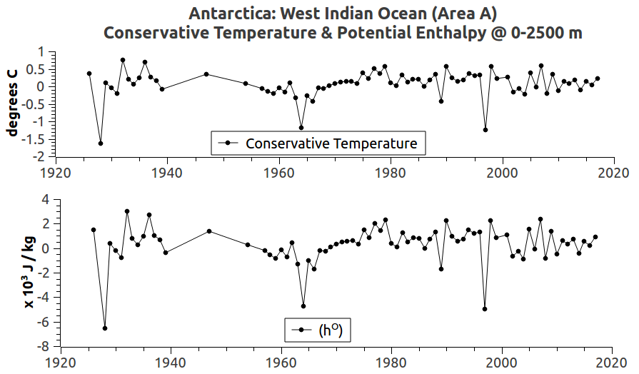
Fig. 3a West Indian Ocean (Area A)
Fig. 3b East Indian Ocean (Area B)
Fig. 3c Ross Sea (Area C)
Fig. 3d Amundsen Sea (Area D)
Fig. 3e Bellingshausen Sea (Area E)
Fig. 3f Weddell Sea (Area F)
The "areas" that the current flows through (Fig. 1 A-F) are graphed in Fig. 3a - Fig. 3f.
Those graphs show that Conservative Temperature (Θ) and Potential Enthalpy (hO) have the exact same pattern.
They have the same thermodynamic proportionality even though they have different values, plus one is temperature ( deg. C ) while the other is Joules per kilogram ( J / kg ).
Those patterns are made from in situ measurements stored in the World Ocean Database (WOD) that are calculated into Conservative Temperature (Θ) and Potential Enthalpy (hO) using the TEOS-10 toolbox.
The combined in situ measurements were taken at depths from 0 m to 2500 m for each of the zones in layers 15-17.
The depths are limited to that range because a tidewater glacier's ice face doesn't go down below sea level to that depth (2500 m) very often, if ever.
What is so interesting to me is that the graphs show that the heat flux is due to a general increase in heat content (hO) around Antarctica.
That heat content is finding its way to the tidewater glaciers, and is melting them from the glaciers' grounding lines all the way up to and along the bottom of the floating ice shelves.
I have shown in other posts that the increasing heat content is also found at even deeper depths there.
However, since my focus is on the danger that the melting glaciers pose to seaports (The Extinction of Robust Sea Ports, 2, 3, 4, 5, 6, 7, 8, 9) I have only shown the shallow tidewater depths today (0-2500m).
Furthermore, the main purpose of today's post is to show the thermodynamic proportionality between CT and hO as harbingers of heat flux.
IV. Conclusion
As Dr. McDougall pointed out, the ocean models will continue to have errors in their heat content and heat flux computations until they replace "potential temperature" with Conservative Temperature.
While their programmers are doing that, adding Absolute Salinity and Potential Enthalpy computations a la TEOS-10 would also be steps in the direction of fewer errors.
The next post in this series is here, the previous post in this series is here.
In this series we have been focusing on the trinity that has brought down some 26 civilizations which came and went (some went down centuries prior to our current civilization).
Of those prior civilizations it has been noted that "... the civilizations then sank owing to the sins of nationalism, militarism, and the tyranny of a despotic minority" (How To Identify The Despotic Minority - 6).
Tyranny by a despotic minority can only be prevented by a ubiquitous free press leading to a well informed populace.
In the embryonic writings of our constitutional republic we see the notion of a "free press" (First Amendment).
That amendment was written prior to the outbreak of corporate media, which is decidedly not a free press now, because it is in varying degrees entangled with commercialism (Corp Germ > Corp Seed > Corp Monster, 2, 3, 4).
II. Mourning Java
This very morning, Morning Joe expanded upon the paranoia that MOMCOM has been spreading concerning what JoJo likes to call "social media" ("unsocial media" would be more accurate).
Thus, McTell News (Blind Willie McTell News, 2, 3, 4, 5, 6) is blundering through yet another revelation that "social media" carries harmful entities (Russian bots) as well as helpful entities (real good and real bad news).
After all, the "air waves" and the actual atmosphere carry both harmful virus and harmful biotic entities, as well as carrying helpful virus and helpful biotic entities (e.g. Etiology of Social Dementia - 5, The Deceit Business).
We can live in the air of this planet, so why can't we live with the "air waves" in social media (The Citizen Journalist In America, 2, 3) ?
III. Despots Anonymous
The despotic minority is composed of both geniuses and dumbbells, males and females, multiple races, and multiple good and bad political entities (How To Identify The Despotic Minority, 2, 3, 4, 5, 6).
Thus, social media culture is very much like the atmosphere and the corporate media.
Corporate media needs to realize that the antidote is a proper educational system loaded with healthy civics, not a whiny corporate media fed with the advertising toxins of MOMCOM.
That educational need also includes a very healthy dose of global warming induced climate change reporting (MOMCOM's Mass Suicide & Murder Pact, 2, 3, 4, 5).
The next post in this series is here, the previous post in this series is here.
In the run-up to TEOS-10, which has been adopted by scientific bodies around the world as the new official standard, some key scientists pointed out why the new standard was preferred over the error prone old standard.
In today's post I want to review the reasons for the change, while showing how the "new parts" synchronize with the new whole.
By "review" I only mean that I will quote Dr. Trevor J. McDougall's paper in a slightly different way in order to focus on the errors in the old standard that were eradicated from the new standard for thermodynamics in oceanography.
I want to focus on the pattern of synchronization between Conservative Temperature and Potential Enthalpy.
As we will see, another valid way of saying that is "the pattern of synchronization between Conservative Temperature and Heat Flux" in seawater, because the old standard "Potential Temperature" was replaced with the new standard "Conservative Temperature" for reasons pointed out in the following quote:
Fig. 2a Epipelagic
Fig. 2b Mesopelagic
Fig. 2c Bathypelagic
Fig. 2d Abyssopelagic
Fig. 2e Hadopelagic
"Potential temperature is used in oceanography as though it is a conservative variable like salinity; however, turbulent mixing processes conserve enthalpy and usually destroy potential temperature. This negative production of potential temperature is similar in magnitude to the well-known production of entropy that always occurs during mixing processes. Here it is shown that potential enthalpy—the enthalpy that a water parcel would have if raised adiabatically and without exchange of salt to the sea surface—is more conservative than potential temperature by two orders of magnitude. Furthermore, it is shown that a flux of potential enthalpy can be called “the heat flux” even though potential enthalpy is undefined up to a linear function of salinity. The exchange of heat across the sea surface is identically the flux of potential enthalpy. This same flux is not proportional to the flux of potential temperature because of variations in heat capacity of up to 5%. The geothermal heat flux across the ocean floor is also approximately the flux of potential enthalpy with an error of no more that 0.15%. These results prove that potential enthalpy is the quantity whose advection and diffusion is equivalent to advection and diffusion of “heat” in the ocean. That is, it is proven that to very high accuracy, the first law of thermodynamics in the ocean is the conservation equation of potential enthalpy. It is shown that potential enthalpy is to be preferred over the Bernoulli function. A new temperature variable called “conservative temperature” is advanced that is simply proportional to potential enthalpy. It is shown that present ocean models contain typical errors of 0.1°C and maximum errors of 1.4°C in their temperature because of the neglect of the nonconservative production of potential temperature ... and potential temperature, rests on an incorrect theoretical foundation ..."
Today's graphs confirm Dr. McDougall's statement that Conservative Temperature (CT) is proportional to Potential Enthalpy (hO) at all pelagic depths (see the link at Fig. 1 for more about pelagic depths).
The graphs at Fig. 2a - Fig. 2e show that the "pattern" of CT, hO, and changes in hO, are identical patterns to one another at all depths.
By pattern I mean that there is a distinct proportionality to those three graph lines even though the value of CT is degrees C, and the values of Potential Enthalpy and change in Potential Enthalpy are shown in Joules per kilogram.
The proportionality pattern indicates that Conservative Temperature is better related to heat content and heat flux than the former potential temperature was.
The graphs at Fig. 3a and Fig. 3b show the same pattern proportionality in a different graph format.
You may have noticed that Absolute Salinity (SA) does not have the same pattern, nor should it.
According to some modelers ocean models are slow to adapt the new standard that was officially released in 2010 (some eight years ago).
Albert Einstein said that when researching and reporting on scientific matters we should "make things as simple as possible, but no simpler" and Dr. Jerry Mitrovica said "the best physics is the simplest physics."
Since we are talking physics when we talk about the laws of thermodynamics at play in seawater, as regular readers know, we are talking about why I use the TEOS-10 software toolbox:
"In 2010, the Intergovernmental Oceanographic Commission (IOC), International Association for the Physical Sciences of the Oceans (IAPSO) and the Scientific Committee on Oceanic Research (SCOR) jointly adopted a new standard for the calculation of the thermodynamic properties of seawater. This new standard, now also endorsed by the International Union of Geodesy and Geophysics (IUGG), is called TEOS-10 and supercedes the old EOS-80 standard which has been in place for 30 years. It should henceforth be the primary means by which the properties of seawater are estimated."
(TEOS-10 Primer, p. 2 PDF, emphasis added). For an extensive elaboration on TEOS-10, see also: McDougall, T.J. and P.M. Barker, 2011: Getting started with TEOS-10 and the Gibbs Seawater (GSW) Oceanographic Toolbox, 28pp., SCOR/IAPSO WG127, ISBN 978-0-646-55621-5.
As I explained in the first post of this series, the TEOS-10 toolbox offers a very simple way of determining heat content, in terms of computer software functions:
The potential enthalpy (hO) is calculated as specific enthalpy (h) minus dynamic enthalpy (h‡) using two TEOS-10 functions:
(In Search Of Ocean Heat). Since that is simple physics, according to those far more knowledgeable than I am, it is the best physics.
III. How Not To Search For Ocean Heat Content
The simple approach has not generally been followed in scientific papers when the authors are researching and reporting on the thermodynamics of seawater.
For an example, a recent paper measured atmospheric characteristics ("the air") ostensibly to determine ocean heat content (On Resplandy Et Alia (2018), 2).
Some less egregious, but nevertheless the long way home examples, are:
"The projected ocean heat uptake (OHU, i.e., the increase in ocean heat content) in model simulations with an increasing CO2 content has a distinct regional structure. We analyse this for the CMIP3 SRES A1B scenario, for which we have the largest number of models available. For comparison, the same analysis for the 1% CO2 runs of CMIP3 and CMIP5 can be found in the auxiliary material. They show generally less heat uptake because ∫F dt is smaller, but the geographical features are similar." (Ocean heat uptake and its consequences for the magnitude of sea level rise and climate change, cf Study Evaluates Efficiency of Oceans as Heat Sink, Gas Sponge).
"Conduction, Convection, and Radiation Oceans are critically important in the movement of heat over the planet. In elementary school you learned that heat moves by conduction, convection, and radiation. Radiation and conduction are effective in moving heat vertically from the earth's surface, but are relatively unimportant in moving heat horizontally. Water, like air, is a fluid that can carry heat as it moves from one place to another. Meteorologists have different terms for horizontal and vertical movement of fluids: movement in the vertical direction driven by buoyancy is called convection, and movement in the horizontal direction is called advection. Convection contributes, with radiation and conduction, to the movement of heat in the vertical direction. But advection is essentially the sole process by which heat moves laterally over the surface of the earth. ... Water Transport of Heat Water is about 1,000 times as dense as air, and, since the amount of thermal energy transported by a moving fluid is proportional to its density, a volume of water can transport about a thousand times as much heat as an equivalent volume of air. The rate at which heat is transported, called the heat flux, is measured in Joules of energy per unit area per unit time, so the rate at which heat is transported is also proportional to the speed of movement (wind speed in air or current speed in the ocean). Since wind speed is typically on the order of 10 meters per second and ocean drift currents on the order of centimeters per second, the air speed is about a thousand times larger than ocean speed. Therefore, air moves a thousand times faster than water but carries only about 1/1000 as much heat per unit volume, which suggests that water is approximately of equal importance to air in moving heat over the planet." (Ocean Structure and Circulation).
The basic error, IMO, which these papers exhibit is to ignore "the world according to measurements" and TEOS-10.
I mean ignoring in situ measurements taken and thereafter processed using the official thermodynamics toolbox, relying instead on "old timey" models and assumed data values.
That is why I ask: "Where da measurements at?"
Fig. 3a
Fig. 3b
Fig. 3c
Fig. 3d
Fig. 3e
IV. How To Search For Ocean Heat Content
In the previous two posts of this series we looked at the mean average of actual heat content values (hO) of the seawater.
Those values are expressed in terms of Joules per kilogram (J / kg), but today we take a new look by calculating only the mean average change in heat content that is taking place annually (still using J / kg of course).
Using the TEOS-10 toolkit, that new look simply means graphing an increase or a decrease in heat content per mass unit of seawater at various depths (Fig. 2) in various latitude bands (Fig. 1) across the oceans of the globe.
This means that today we are not graphing the actual values, instead, we are graphing the change in actual values from one year to the next.
That allows us to track "heat" that is driven by the laws of thermodynamics as that heat radiates through the ocean depths.
V. The Graphs Generally
As was done in the previous posts in this series, the layers marked with blue squares at Fig. 1 are the specific layers we are examining.
The graph values all start at zero change for the first measurement, then increase or decrease as TEOS-10 functions determine the heat content changes (Section II above).
Changes in heat content show that over time heat has radiated into or radiated out from seawater at various depths at those latitude band locations.
Furthermore, the graphs which show the Hadopelagic depth changes inform us that the heat content changes are radiating all the way down to the deepest depths.
Even though the deepest depth regions have not been measured as extensively (to say the least) as the upper depth levels have been, we can still see that heat content change reaches down to the deepest depths.
It is worthwhile to know that the in situ measurements processed into TEOS-10 values show that the heat content down there, like the depth levels above it, is also in flux.
Assuming that you have built your system, constructing the heat flux graphs only involves:
1) selecting a year to begin with,
2) setting the begin-year initial change value to zero,
3) recording that initial value, and thereafter
4) subtracting that initial value from each following year's value,
5) graphing the change in heat content for each year.
The graphs will leave a "fingerprint" of the heat flux over the span of the years chosen to be graphed and studied.
VI. The Graphs: Specifically
A. Fig. 3a
The graph at Fig. 3a details the changes in potential enthalpy (hO), a.k.a. "heat content" and heat flux at WOD Layer 0 (Arctic seawater, see graph Fig. 3a here).
The sequence begins circa 1950 with a change value of zero J / kg.
Then the fun begins as we examine the fingerprints of the culprit we call "the heat" for the following years.
At this layer over this span of about 70 years, heat content decreases at the Epipelagic and Mesopelagic depth levels, but increases at the Bathypelagic depth level.
In other words the heat is obeying the 2nd law of thermodynamics (heat spontaneously flows to cold).
B. Fig. 3b
This layer 4 is at the latitude that crosses portions of the USA, Europe, and China.
The latitude layers away from the poles tend to have deeper waters, so we even have some Hadopelagic measurements and values at WOD Layer 4.
Comparing this change in heat content with the actual heat content graphs shows how the heat flux graphs tell us even more about heat content dynamics in the oceans (see graph Fig. 3b here).
A point to take note of is that each downward direction on each graph line tells us that heat radiated out of seawater at that level, while each upward direction on each graph line tells us that heat radiated into the seawater at that level.
So, we have direct evidence of heat flux into and out of seawater at all depths of the ocean along this latitude.
I noticed that, counter intuitively, the deepest level, the Hadopelagic, had more heat flux at times than shallower levels had.
This is a good time to remember that heat flux can be greater in one depth level even though that depth level can at the same time have less actual heat content than that other level which had more heat flux (i.e. the amount of change in potential enthalpy (hO) does not ipso facto indicate the total amount of potential enthalpy (hO) contained in that particular mass unit of seawater).
C. Fig. 3c
This WOD layer 8 has one boundary we call the Equator (latitude 0).
The heat flux here is also "at odds" with the total heat content (see graph Fig. 3c here).
D. Fig. 3d
The latitude of WOD Layer 12 crosses Australia (etc.).
The ocean at that latitude has some Hadopelagic depths.
An interesting tidbit is that its Epipelagic level has the most heat flux at times, indicating either heat flux radiating down from solar energy or radiating up from a sometimes warmer Mesopelagic level.
One case in point is the year 1997 where the Mesopelagic level just under it (red line) has a severe decrease in heat content when the Epipelagic had a sharp increase (compare Fig. 3d here).
The gist of heat flux, in terms of graph lines, is that when the line dips downward heat content at that level has radiated to another level, and when the graph line turns upward, it indicates some heat content from another level has radiated into that level.
In all cases, the radiation can come from below or from above, whether the change is an increase or a decrease.
E. Fig. 3e
This is WOD Layer 16 which circles Antarctica.
The greatest current on Earth flows in this layer, containing more flow of seawater than the fresh water flow in all of the Earth's great land-based rivers combined.
Like the Arctic, it does not have the Hadopelagic depth level.
It has some of the other characteristics of the Arctic, in that the deeper depths tend to show increases in heat flux in recent years.
Also, the heat content at the surface varies with heat flux (see Fig. 3e here).
VII. Conclusion
Heat flux means a change in heat content in a mass unit of seawater.
Graphs of actual heat content (hO, potential enthalpy) do not show heat flux as clearly as change in hO graphs used along with them do.
Using both together produces the best results, because both used together offer substantial support for a better understanding of heat content vs heat flux in all of the ocean basins (cf. Patterns: Conservative Temperature & Potential Enthalpy).
The next post in this series is here, the previous post in this series is here.
Must we? ...