 |
| Fig. 1 |
I. Background
In a recent post I indicated that a new software module I am developing had not yet been finished, even though I was presenting some output from the beta version of that module I was still working on.
That new module is focused on three depth layers, like previous Dredd Blog software had been (The Layered Approach To Big Water - 9).
 |
| Fig. 2a |
 |
| Fig. 2b |
 |
| Fig. 2c |
 |
| Fig. 2d |
So, today, I am presenting the portion that was not, at that time, finished.
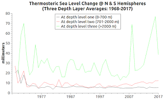
NOTE: this new model uses only paired measurements, which are salinity (SP) and temperature (T) measurements taken at the same time, place, and depth (some previous Dredd Blog graphs were generated using all WOD measurements regardless of pairs).
Anyway, the new module focuses on thermal expansion and contraction of those three depth layers.
The geographical locations are the same (N. Hemisphere, S. Hemisphere, and Global Mean Average).
The global mean average is simply a combination of the two hemispheres.
The graph at Fig. 1 (upper left pane) shows tide gauge measured sea level change over the years 1968-2017.
The upper right pane, and the two lower panes show the mean average versions of thermal expansion and/or contraction over that same period of time.
The bottom line totals for those Fig. 1 thermosteric volume changes are:
NH begin: = 15.9879
NH end: 28.9791
----------------------------------
net: 12.9912 mm
SH begin: 31.2034
SH end: 8.65903
----------------------------------
net: −22.54437
(−22.54437 + 12.9912) ÷ 2 = −4.7766
Mean Begin: 23.5956
Mean end: 18.819
18.819−23.5956 = −4.7766
In other words, the global mean for pairs indicates a negative volume change of 4.7766 mm over that span of time (nevertheless, sea level is rising).
The graphs at Fig. 2a - Fig. 2d show the thermal expansion and/or contraction at the three depths in the aforementioned hemispheres as well as in the global mean of those hemispheres and depths.
The point of it is that there is variance in thermosteric volume change at various depth layers in the hemispheres and in the global mean.
The graphs show that sometimes the deeper layers have more action in that regard than the upper layers do.
II. More Evidence For Cold Sea Water Melting Sea Ice
In addition to that, I found a paper which uses the TEOS-10 toolkit that I also use (Melting of Ice and Sea Ice into Seawater and Frazil Ice Formation, PDF).
That paper is very technical, dealing with sea water and sea ice at or very near the freezing point.
In so doing, it mentions the following TEOS-10 toolkit functions:
gsw_CT_from_tI mention this paper because I criticized the habit of calling the sea water "hot" that melts the most sea ice when describing a Chinese scientific paper that had called it "warm" (Questionable "Scientific" Papers - 17).
gsw_frazil_ratios
gsw_CT_freezing_poly
gsw_CT_from_pt
gsw_t_freezing_first_derivatives
gsw_melting_ice_into_seawater
gsw_melting_ice_SA_CT_ratio
gsw_CT_freezing_first_derivatives
gsw_ice_fraction_to_freeze_seawater
gsw_melting_ice_equilibrium_SA_CT_ratio
gsw_enthalpy_first_derivatives_CT_exact
The reality is that both the Chinese and the Americans who wrote about it were puffing.
The highly scientific TEOS-10 source code comments place the word in quotes ("warm") when talking about very cold sea water temperatures that melt sea ice.
So, today I am going to elaborate on the TEOS-10 toolkit function "gsw_melting_ice_into_seawater" (gsw_melting_ice_into_seawater) in the hopes that it will shake some of the warming commentariat out of their trance (The Warming Science Commentariat, 2, 3, 4, 5, 6, 7, 8, 9, 10, 11; cf. Climate Feedback).
III. The Temperate Reality
In preparing for future posts that will point out places where very cold water is melting sea ice, I am writing a module specifically for that purpose, again, based on the "gsw_melting_ice_into_seawater" function of the toolkit.
The purpose of this exercise is to remind us that very little global warming can increase the temperature of cold, deep ocean waters just a little bit and still cause the melting of the ice sheets, ice shelves, and the land glaciers that protrude into ocean waters.
The following C++ program utilizes the TEOS-10 function "gsw_melting_ice_into_seawater" to calculate sea ice melting into water and the temperature of that same sea water that melted the ice:
#include <iostream>
#include <fstream>
#include <iomanip>
/** TEOS header file */
#include <gswteos-10 .h>
using namespace std;
/** values taken from TEOS-10 website */
const unsigned maxValues = 6;
const double SA[maxValues] ={34.7118,34.8915,35.0256,34.8472,34.7366,34.7324};
const double CT[maxValues] = {4.7856,2.4329,1.8103,1.2600,0.6886,0.4403};
const double P[maxValues] = {10,50,125,250,600,1000};
const double W_Ih[maxValues] = {0.0560,0.02513,0.02159,0.01210,0.00943,0.00751};
const double T_Ih[maxValues] = {-4.7856,-4.4329,-3.8103,-4.2600,-3.8863,-3.4036};
const char *txtFile = "icemelt.txt";
int main()
{
freopen(txtFile, "w", stdout);
for (unsigned cpos = 0; cpos < maxValues; cpos++)
{
/** input */
double sa = SA[cpos], ct = CT[cpos], p = P[cpos];
double w_ih = W_Ih[cpos], t_ih = T_Ih[cpos];
/** output */
double sa_final, ct_final, w_ih_final;
gsw_melting_ice_into_seawater(sa, ct, p, w_ih, t_ih,
&sa_final,
&ct_final,
&w_ih_final);
cout << setprecision(15)
<< sa_final << "\t"
<< ct_final << "\t"
<< w_ih_final << endl;
}
return 0;
}
The program prints this into the file:
[SP] [CT] [w_ih]
32.7679392 -0.298448911022612 0
34.014676605 0.215263001418312 0
34.269397296 -0.074341719211558 0
34.42554888 0.207796293045473 0
34.409033862 -0.123785388299875 0
34.471559676 -0.202531182809225 0
Those results are what the toolkit EXAMPLE indicates (gsw_melting_ice_into_seawater).
Note that the numbers in red are the sea water temperatures before and after melting.
The temperatures (CT) are degrees Celsius (4.7856 C = 40.61408 F, 0.4403 C = 32.79254 F).
Those "hot" temperatures can be life threating:
Hypothermia can occur when you are exposed to ... 60°F (16°C) to 70°F (21°C) water [OR COLDER].(WebMD). So, water "warm" or "hot" enough to melt subsurface ice sheets or ice shelves is actually cold enough to kill you if you are submerged in it long enough.
IV. Conclusion
Let's not be like the deniers, let's not get hyperbolic or hypothermia.
The next post in this series is here, the previous post in this series is here.


