On Thermal Expansion & Thermal Contraction - 28

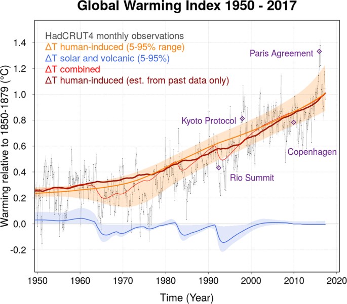
Fig. 1 Nature Global Warming Index

In the previous post of this series I mentioned a new software module which I was constructing.

I indicated that it is designed to assist with selecting sample World Ocean Database (WOD) areas to use as representing what is generally happening to the oceans as a whole (On Thermal Expansion & Thermal Contraction - 27).

I even began a new series to describe the progress with that project (Oceans: Abstract Values vs. Measured Values, 2, 3).

The subject matter involved, sometimes called "cherry picking" and sometimes called "selection bias," is relevant to not only thermal expansion theory, but is relevant to any issue that relates to global mean averages of ocean temperature and salinity.

A recent paper "A real-time Global Warming Index" published in Nature (link at Fig. 1) discusses some of the issues regarding the selection of data sources regarding air temperature changes over the years.

Fig. 2 All about the surface

Another paper from years ago discusses the issues regarding selection of tide gauge stations that reasonably represent global mean sea level rise (Global sea level rise).

Yet another paper goes through the paces concerning ocean temperature and salinity measurements (Objective analysis of monthly temperature and salinity for the world ocean in the 21st century: Comparison with World Ocean Atlas and application to assimilation validation, PDF);

Fig. 3a

Fig. 3b

Fig. 3c

Fig. 3d

Fig. 3e

Fig. 3f

The graph at Fig. 2 shows the ocean surface anomaly which has a similar trend to the anomaly of air temperatures shown in Fig. 1.

But I haven't found a discussion of a global mean based on proper locations of measurements.

Measurements chosen so that they render a balanced overall view (such as GISTEMP).

One paper discusses the mean (A monthly mean dataset of global oceanic temperatureand salinity derived from Argo float observations, PDF).

In that paper they talk about not being able to use certain datasets because of various degrees of lack of uniformity.

But, like the old problem with tide gauge station measurements that caused consternation before Bruce C. Douglas set forth the Golden 23, the quality of the measurements is not the problem.

The problem is which WOD zones or layers to use as a representation of the whole.

Until that is done, including all depth measurements available down below the 2,000 m mark, calculating thermal expansion seems baseless.

The software module (version 1.5) now uses several combinations of WOD layers which prove that selection of WOD Zones is just like selection of PSMSL tide gauge locations.

That is quite obvious in today's graphs which compare: 1) all WOD zones, 2) the Golden Six Layers, 3) an alternate six layers, and 4) an abstract group described at section "II. New Software Module" here.

The graphs in today's post show that any calculations of thermal expansion, or global mean average temperature and salinity changes, cannot competently be set forth unless and until "The Golden" locations are hypothesized and thereafter not falsified.

Temperature (CT), salinity (CT) and thermal expansion all vary according to the areas used to compute those values (see Fig. 3a - Fig. 3f).

The reason why I hypothesize "The Golden Six Layers" as an appropriate selection is that it matches the abstract, the GISTEMP anomaly, and the surface temperature anomaly closely enough to be conducive to providing a reasonable knowledge of what is taking place down under the surface.

The next post in this series is here, the previous post in this series is here.