|
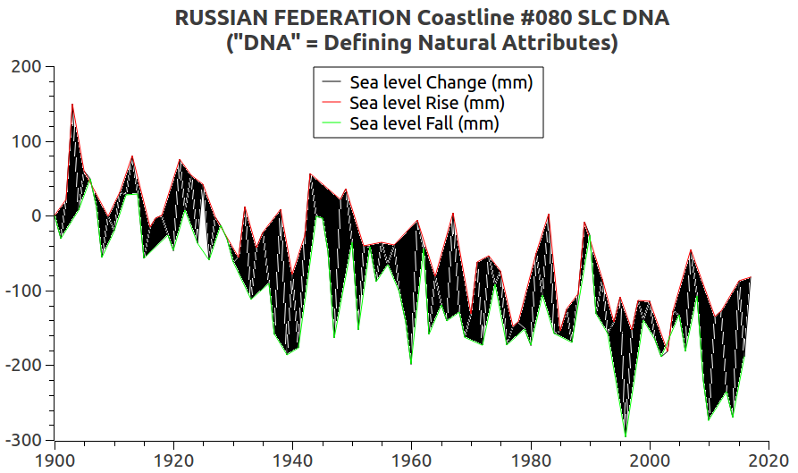
| Fig. 1 |
In today's post I want to detail the concept of sea level change (SLC) "DNA."
I'll start off by quoting from the description in the first post:
I think that "DNA" is also a useful and perhaps better term for the tell-tale indicators of sea level change (SLC).(Beyond Fingerprints: Sea Level DNA). That is only a beginning, so on with the details.
Using "DNA" when referring to the pattern of a geographical location's sea level change (SLC) means its "Defining Natural Attributes" that are the combination of the downward and upward influences over a period of time that is long enough to establish a trend.
Fig. 2
A dictionary meaning of "defining" is:
"a defining feature or characteristic is one that is completely typical of something and allows it to be identified"(Macmillan Dictionary).
A dictionary meaning of "attribute" is:
"a quality or feature of a ... thing, esp. one that is an important part of its nature"(Cambridge Dictionary).
So, I am presenting that notion of sea level DNA as four components of tell-tale indicators, which are: 1) the distances from a tide gauge location to the ice sheet or glacier field locations, 2) the SLC indicator, 3) the SLR indicator, and 4) the SLF indicator.

II. The Beginning Years Compared
The graphs shown in Fig. 1 and Fig. 2 show a different beginning year.
One reason I do that today, is to show that SLC DNA (defining natural attributes) changes with time.
The beginning years in the graph at Fig. 2 relates to the exercise in another post in another series (Appendix to Countries With Sea Level Change - 4) which was comparing thermosteric volume change calculations with tide gauge records.
That difference between Fig. 1 and Fig. 2 is not important to the subject matter of the remainder of this post.
The purpose today is to show how to derive the Fig. 2 results.
But before moving on into that, I should point out how the PSMSL tide gauge station records are used.
The first thing to do is to download the PSMSL data (Complete PSMSL Data Set).
That consists of the annual set and the monthly set (ibid).
Next, I combine the annual with the sum of the monthly, then average the two before finally placing the final results into an SQL server.
III. Building A CSV File
The CSV file shown below was constructed as follows:
1) Assume an array of PSMSL data containing tide gauge records from 1800 to 2019, and a CSV file header with columns "year, RLR, SLC, SLR, SLF".
2) Assume that, in that array, rows that contain no data have a "year" value of zero (0).
3) While progressing through the array in a sequence from the oldest annual record to the most recent annual record, if the year value in the array is not zero, do the following:
1) on the first (oldest) record acquire the year (assume "1910") and RLR ("6970.49") values, (so, 6970.49 - 6970.49, means that the first SLC, SLR, and SLF values will be zero),
2) store the first RLR value as the amount to delete from each subsequent annual RLR value.
3) as you progress through each recorded RLR value:
a) delete the original RLR value from each subsequent year's RLR value to obtain the SLC, then the SLR and SLF,4) for each record following the first record, write the following to the CSV file:
b) the amount resulting from the current RLR minus the orig RLR (e.g. for year 1911) will be 6902.22 - 6970.49) which is the sea level change (SLC) value,
c) after the deletion on the first record, store, in the CSV file, the year value (e.g. 1910), the RLR value (e.g. 6970.49), the SLC value (0), SLR value (0), and the SLF value (0).
a) if the RLR value is greater than the one preceding it, write the change value to the SLR column, but leave the SLF column empty (not zero ... notice the rows ending in a comma, denoting an empty SLF value)An example CSV file which results from the above process:
b) if the RLR value is less than the one preceding it, write the change value to the SLF column, but leave the SLR column empty (",,").
year, RLR, SLC, SLR, SLFOn the final row I write the change value (current RLR minus the orig RLR) in all the columns (i.e. the SLC, SLR, and SLF columns).
1910,6970.49,0,0,0
1911,6902.22,-68.2708,,-68.2708
1912,6920.84,-49.6457,-49.6457,
1913,6927.92,-42.5725,-42.5725,
1914,6932.51,-37.9766,-37.9766,
1915,6944.09,-26.3986,-26.3986,
1916,6945.48,-25.0123,-25.0123,
1917,6953.66,-16.8307,-16.8307,
1918,6960.77,-9.72447,-9.72447,
1919,6983.79,13.2975,13.2975,
1920,6947.99,-22.5021,,-22.5021
1921,6968.84,-1.65338,-1.65338,
1922,6933.69,-36.8018,,-36.8018
1923,6921,-49.4864,,-49.4864
1924,6934.27,-36.2217,-36.2217,
1925,6919.23,-51.2643,,-51.2643
1926,6912.6,-57.8896,,-57.8896
1927,6930.75,-39.7431,-39.7431,
1928,6915.95,-54.5442,,-54.5442
1929,6910.22,-60.2736,,-60.2736
1930,6908.17,-62.3202,,-62.3202
1931,6897.97,-72.5198,,-72.5198
1932,6917.49,-53.0008,-53.0008,
1933,6942.17,-28.3243,-28.3243,
1934,6888.42,-82.069,,-82.069
1935,6919.65,-50.8394,-50.8394,
1936,6932.29,-38.1967,-38.1967,
1937,6951.43,-19.0565,-19.0565,
1938,6954.79,-15.6985,-15.6985,
1939,6947.71,-22.7761,,-22.7761
1940,6952.03,-18.4609,-18.4609,
1941,6938.19,-32.302,,-32.302
1942,6965.56,-4.93051,-4.93051,
1943,6961.84,-8.65367,,-8.65367
1944,6970.09,-0.397266,-0.397266,
1945,6996.51,26.0242,26.0242,
1946,6998.45,27.9626,27.9626,
1947,7007.88,37.3935,37.3935,
1948,7030.66,60.1675,60.1675,
1949,6987.08,16.5885,,16.5885
1950,6961.46,-9.0315,,-9.0315
1951,7000.73,30.2366,30.2366,
1952,6999.24,28.75,,28.75
1953,7001.52,31.0328,31.0328,
1954,6989.53,19.0432,,19.0432
1955,7003.41,32.9182,32.9182,
1956,6998.64,28.1464,,28.1464
1957,6999.31,28.8244,28.8244,
1958,7024.97,54.484,54.484,
1959,6983.24,12.7457,,12.7457
1960,7034.26,63.772,63.772,
1961,7015.59,45.0957,,45.0957
1962,7014.62,44.1298,,44.1298
1963,6975.73,5.24305,,5.24305
1964,6975.09,4.60036,,4.60036
1965,6980.01,9.51824,9.51824,
1966,6998.02,27.5288,27.5288,
1967,7002.83,32.3448,32.3448,
1968,6987.32,16.8295,,16.8295
1969,7024.7,54.2094,54.2094,
1970,7029.06,58.5714,58.5714,
1971,7024.42,53.9325,,53.9325
1972,7050.43,79.9438,79.9438,
1973,7045,74.5061,,74.5061
1974,7014.63,44.1406,,44.1406
1975,7035.82,65.3341,65.3341,
1976,6994.87,24.3809,,24.3809
1977,7005.75,35.2557,35.2557,
1978,7023.17,52.6759,52.6759,
1979,7005.99,35.5043,,35.5043
1980,6997.75,27.2631,,27.2631
1981,7007.45,36.9562,36.9562,
1982,7003.93,33.4353,,33.4353
1983,7073.28,102.793,102.793,
1984,7046.36,75.8648,,75.8648
1985,7024.55,54.0607,,54.0607
1986,7029.04,58.5524,58.5524,
1987,7036.54,66.0527,66.0527,
1988,7009.18,38.6854,,38.6854
1989,7000.76,30.2655,,30.2655
1990,7016.34,45.8516,45.8516,
1991,7058.11,87.6236,87.6236,
1992,7057.05,86.5557,,86.5557
1993,7063.01,92.5238,92.5238,
1994,7044.87,74.3832,,74.3832
1995,7068.58,98.0887,98.0887,
1996,7083.65,113.155,113.155,
1997,7091.34,120.853,120.853,
1998,7109.94,139.448,139.448,
1999,7081.16,110.671,,110.671
2000,7067.27,96.7803,,96.7803
2001,7057.81,87.32,,87.32
2002,7060.7,90.2074,90.2074,
2003,7073.77,103.278,103.278,
2004,7066.97,96.4806,,96.4806
2005,7112.91,142.42,142.42,
2006,7091.71,121.22,,121.22
2007,7069.33,98.8381,,98.8381
2008,7088.95,118.463,118.463,
2009,7121.87,151.383,151.383,
2010,7136.69,166.202,166.202,
2011,7126.23,155.739,,155.739
2012,7129.18,158.693,158.693,
2013,7120.54,150.052,,150.052
2014,7132.87,162.378,162.378,
2015,7123.26,152.769,,152.769
2016,7159.06,188.572,188.572,
2017,7151.32,180.833,,180.833
2018,7172.42,201.928,201.928,201.928
But that is not absolutely required, you can treat the final row like previous rows in the CSV file.
That would render the final row as "2018,7172.42,201.928,,201.928".
The SciDavis graphing program (free), is what I use to generate the graphs displayed on Dredd Blog.
In line graphs, as in the configuration discussed above, by default SciDavis writes the lines in different colors (SLC in black, SLR in red, and SLF in green as shown in Fig. 1).
Which color that results on which line is determined by the column sequence (in the CSV file) you choose to graph with SciDavis.
IV. The DNA Result
The final effort is to fill in the white/empty spaces between the red and green lines with black as shown in Fig. 2.
I use KolourPaint (free) to do that.
This results in a stark depiction of the defining natural attributes of the SLC in the country / coastal area where the PSMSL data was recorded.
The results are composed totally of in situ data (the world according to measurements, not models).
V. Today's Appendices
The Fig. 2 format was generated in graphs for each country that has two or more PSMSL coastline values.
Links to today's main body of graphs are as follows: graphs of countries are listed in alphabetically oriented appendices: A-C, D-G, H-L, M-O, P-T, and U-Y.
VI. Closing Comments
The Antarctica and Greenland Ice Sheet mass loss has increased six fold or so in recent decades (Forty-six years of Greenland Ice Sheet mass balance from 1972 to 2018, Four decades of Antarctic Ice Sheet mass balance from 1979–2017).
Thus, for local SLC response planners it is all the more important to know how their area will be impacted (SLC DNA "Defining Natural Attributes" will be helpful as it is developed into robustness).
This post is a public service of Dredd Blog (The media are complacent while the world burns).
The next post in this series is here, the previous post in this series is here.