Saturday, January 27, 2024

When Heat Hides Under The Refrigerator

Fig. 1 The heat down under

The old song 'Looking For Love In All The Wrong Places' has scientific relevance if we change the name of the song to 'Looking For Heat In All The Wrong Places'.

That has been clearly pointed out in the Dredd Blog series In Search Of Ocean Heat, 2, 3, 4, 5, 6, 7, 8, 9, 10, 11, 12, 13, 14.

Cosmic legislation found in the law of thermodynamics (heat law) indicates that warm/hot flows to cool/cold ("The Second Law of Thermodynamics(first expression): Heat transfer occurs spontaneously from higher- to lower-temperature bodies but never spontaneously in the reverse direction.").

Since the ocean is within the jurisdiction of the cosmos, that law (2nd law of thermodynamics) applies to the oceans of the Earth.

If Sherlock Holmes was on the case he would say look for heat transfer, i.e. moving heat flowing from warm/hot to cool/cold, and follow it to the place it is headed to.

All of the billions of dollars spent on satellites that measure the surface temperature of the ocean (Sea Surface Temperature) won't solve the case, because the 'who dunnit' was and still is The Ghost Photons.

Those "wiley wascals" have pulled the wool over the eyes of the warming commentariat (The Warming Science Commentariat - 13). 

In short, when one is on the hunt for a suspect, one must know what that suspect is, especially in physics where formulas of solutions are required.

The suspect "ocean heat" is know by the 'nickname' described in a paper in a journal:

"Potential temperature is used in oceanography as though it is a conservative variable like salinity; however, turbulent mixing processes conserve enthalpy and usually destroy potential temperature. This negative production of potential temperature is similar in magnitude to the well-known production of entropy that always occurs during mixing processes. Here it is shown that potential enthalpy—the enthalpy that a water parcel would have if raised adiabatically and without exchange of salt to the sea surface—is more conservative than potential temperature by two orders of magnitude. Furthermore, it is shown that a flux of potential enthalpy can be called “the heat flux even though potential enthalpy is undefined up to a linear function of salinity. The exchange of heat across the sea surface is identically the flux of potential enthalpy. This same flux is not proportional to the flux of potential temperature because of variations in heat capacity of up to 5%. The geothermal heat flux across the ocean floor is also approximately the flux of potential enthalpy with an error of no more that 0.15%. These results prove that potential enthalpy is the quantity whose advection and diffusion is equivalent to advection and diffusion of “heat” in the ocean. That is, it is proven that to very high accuracy, the first law of thermodynamics in the ocean is the conservation equation of potential enthalpy. It is shown that potential enthalpy is to be preferred over the Bernoulli function. A new temperature variable called “conservative temperature” is advanced that is simply proportional to potential enthalpy. It is shown that present ocean models contain typical errors of 0.1°C and maximum errors of 1.4°C in their temperature because of the neglect of the nonconservative production of potential temperature ... and potential temperature, rests on an incorrect theoretical foundation ..."

(Patterns: Conservative Temperature & Potential Enthalpy, quoting Potential Enthalpy: A Conservative Oceanic Variable for Evaluating Heat Content and Heat Fluxes). That post shows that Conservative Temperature (CT) and Potential Enthalpy (Ho) have the same "genes", i.e. the same pattern at all ocean depths and temperatures.

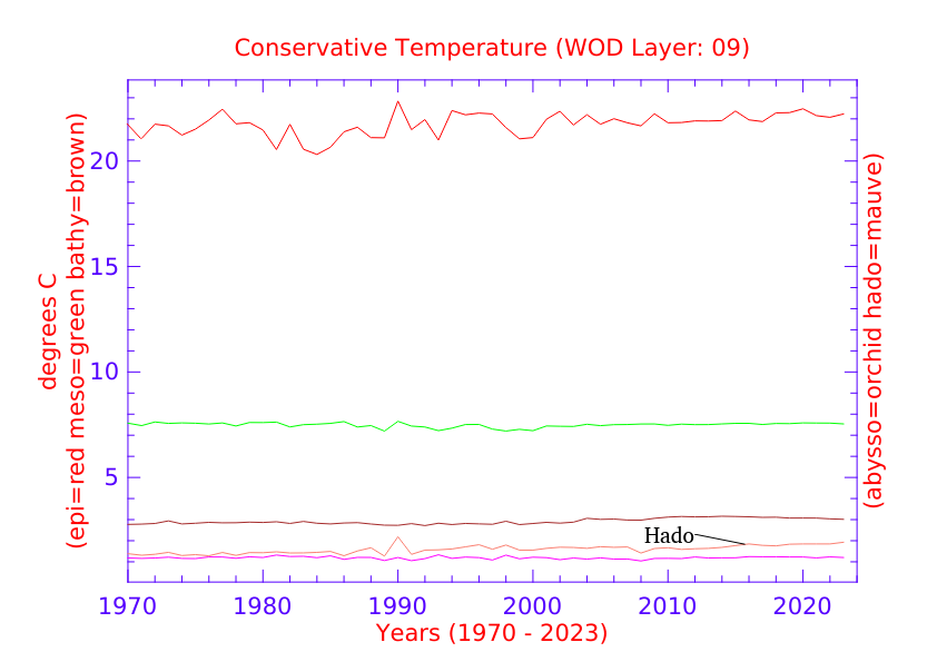
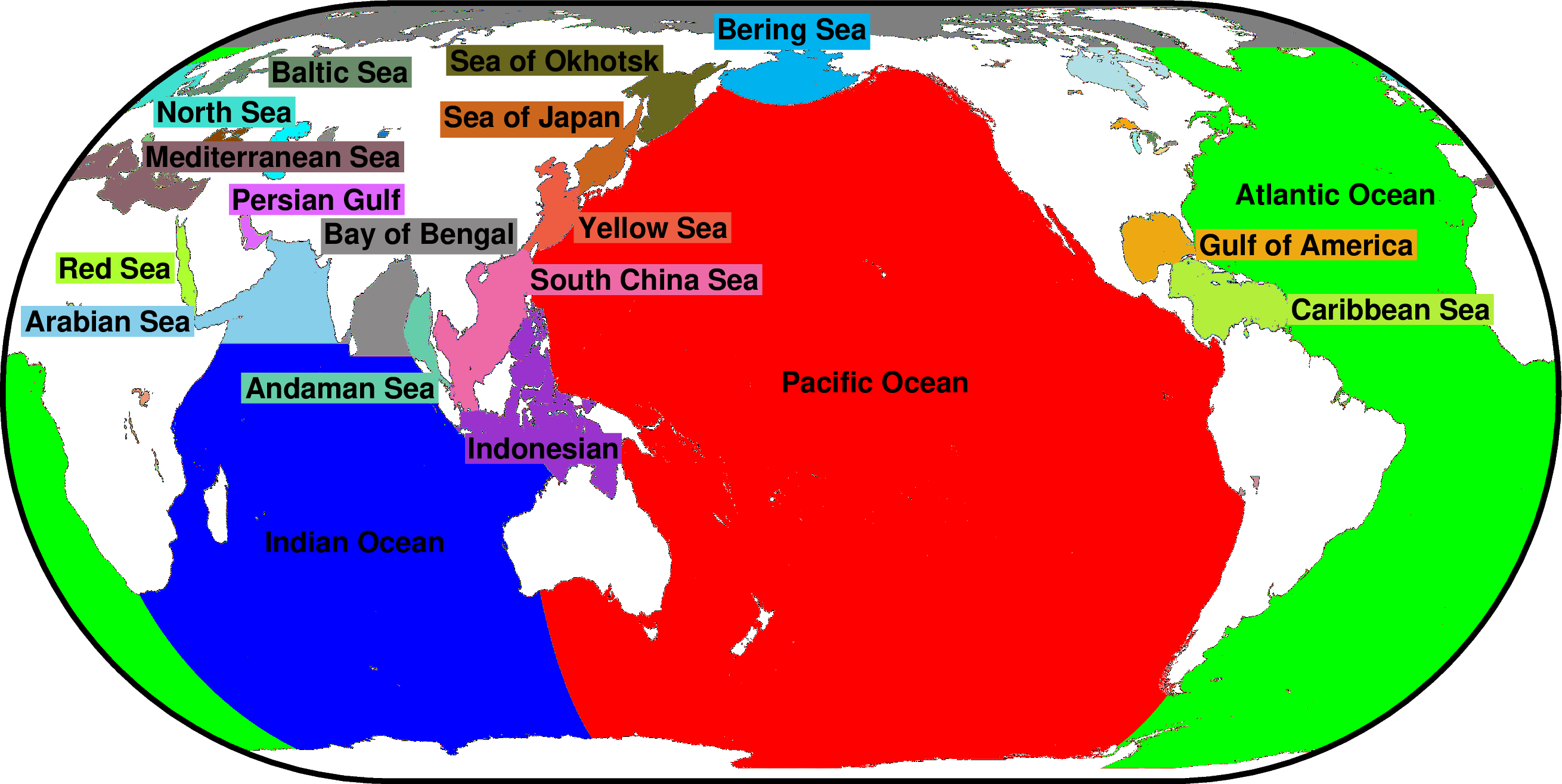
Fig. 2 WOD Zone Layers (red numbers)
In other words "heat" leaves fingerprints that are traceable to those who look deeper than the ocean surface.

The heat flux trail leads to the bottom, the originally coldest place, where the ghost photons have raised the deepest temperatures there to a level above the shallower depth above the deepest level.

The appendices contain graphs which show that the Hadopelagic (deepest level) is becoming warmer than the level above it, the Abyssopelagic (Pelagic zone), and this is not just for WOD ocean layers 14,15, and 16 (Fig. 2) which is the Southern Ocean surrounding "the refrigerator" Antarctica shown in Fig. 1.

The heat flux trip from the surface to the coldest seawater down under has taken decades, but the graphs in the appendices with in situ measurements up to the year 2023, expose the suspect ghost photons at work (Appendix 1, Appendix 2, Appendix 3).

Get on your horse alarmist Paul Revere, and ring them bells Bob Dylan, because "The Hado is Warming" ... "The Hado is Warming".

The big deal about this is that the tidewater glaciers are being melted by heat down under (Antarctica 2.0 - 13).

The next post in this series is here.


"Plug in to the down under ..."


Appendix 3 OHC

This is an appendix to: When Heat Hides Under The Refrigerator


Appendix 2 OHC

This is an appendix to: When Heat Hides Under The Refrigerator


Appendix 1 OHC

This is an appendix to: When Heat Hides Under The Refrigerator


Wednesday, January 24, 2024

On The More Robust Sea Level Computation Techniques - 9

Fig. 1 Ocean Areas

Dredd Blog has used satellite data in sea level change scenarios in the past (On The More Robust Sea Level Computation Techniques, 2, 3, 4, 5, 6, 7, 8).

The most-recent post in this series took place in January of 2017.

So, today I am presenting appendices containing updated satellite records which bring the annual coverage up to the year 2022; but to properly set the stage for the insertion of that satellite data, a comprehensive set of historical PSMSL data is utilized.

I am revisiting this series since there is more satellite data available now, and since the tide gauge station data is decreasing in quantity.

This decrease in quantity is taking place for several reasons mentioned here (notice especially Fig. 4 in that post).

In other words, I have blended the tide gauge station data (beginning circa 1800) with the much more recent satellite data (beginning circa 1992).

I think this approach is required for a stable viewpoint:

"The interest in the use of satellite altimeter data close to the coast motivated a research discipline now referred to as coastal altimetry. Although significant progress has been achieved in the past decades especially in radar technology innovation, development of advanced waveform retracking algorithms, and improved corrections, nonetheless, obtaining accurate sea level from satellite altimetry close to about 5–10 km of the coasts remains a challenge."

(Advances in estimating Sea Level Rise). Sea level data far from coasts is useful, and so is coastal sea levels, because the latter is where the harbors and sea ports are; which is where the heart of international commerce takes place: (Seaports With Sea Level Change, 2, 3, 4, 5, 6, 7, 8, 9, 10, 11, 12, 13, 14, 15, 16, 17, 18, 19, 20, 21, 22, 23, 24, 25, 26, 27, 28, 29, 30, 31, 32, 33).

The graphs presented today are a combination of value lines, with red value lines marking the high and low sea level ranges, blue lines marking the average of the high and low values, and green lines marking the in situ measurements of sea levels.

The most stark differences between these satellite sea level change values and tide gauge record values is that the satellite measurements are not limited to coastlines where tide gauge stations are located.

The satellite measurements are taken at latitude and longitude locations out to the furthest reaches of the oceans way off shore; but they both utilize "the geoid" concept. 

Thus, there are two types of values in today's appendices.

One is the RLR (geoid) millimeters (complicated math calculations) and the other is straight millimeters (simple tide gauge floats moving up and down within a tube):

"In order to construct time series of sea level measurements at eachstation, the monthly and annual means have to be reduced to a common datum. This reduction is performed by the PSMSL making use of the tide gauge datum history provided by the supplying authority. To date, approximately two thirds of the stations in the PSMSL database have had their data adjusted in this way, forming the 'REVISED LOCAL REFERENCE' (or 'RLR' [geoid]) dataset. In general, only RLR data should be used for time series analysis."

(RLR Definition; cf. Ocean surface topography). The straight millimeters value on the graphs is acquired by recording the first RLR sea level value (earliest year) then subtracting that value from all subsequent RLR values to derive the anomaly value (Note that satellite these measurements begin circa 1992 and are the values that replace missing tide gauge station data that have ceased to exist; or authorities have stopped presenting data to PSMSL for some other reason such as sea level change damage done to tide gauge stations).

Anyway, here are the appendices composed of sea level change graphs at various ocean areas within them (ocean names are in alphabetical order: A-C 1800, G-P 1800J-Y 1800; A-C 1992, G-P 1992J-Y 1992).

The '1992' designation indicates measurements containing only the satellite values beginning in 1992 while the '1800' designation indicates measurements of tide gauge values beginning in 1800 with satellite data blended in from 1992 forward.

The previous post in this series is here.


"Now I wish I could write you a melody so plain
That could hold you dear lady from going insane
That could ease you and cool you and cease the pain
Of your useless and pointless knowledge"


Appendix J-Y 1992

This is an appendix to: On The More Robust Sea Level Computation Techniques - 9


Appendix G-P 1992

This is an appendix to: On The More Robust Sea Level Computation Techniques - 9


Appendix A-C 1992

This is an appendix to: On The More Robust Sea Level Computation Techniques - 9


Appendix J-Y 1800

This is an appendix to: On The More Robust Sea Level Computation Techniques - 9