 |
| Fig. 1 |
In the previous post of this series I quoted from a peer-reviewed paper which explained how to calculate change in heating & cooling caused volume change (Thermal expansion & contraction) in seawater (Quantum Oceanography - 15).
Today, I will add to that post with enough detail that you can build your own system to measure thermosteric sea level change, or at least know how it is done properly.
But, I won't repeat the part about getting the copious amounts of data needed to do a thorough exercise (Build Your Own Thermosteric Computational System).
Suffice it to say the paper I critiqued in the previous post did not do a thorough exercise.
Professionalism, when it comes to sea level change research, involves collecting the most important factor, which is the in situ measurements from the most abundant sources (WOD, SOCCOM, WHOI, PSMSL, and OMG).
The data I use from those sources amounts to ~5.5 billion in situ measurements from about 1800 to 2021.
II. The World Ocean Database (Zones & Layers)
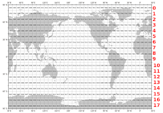 |
| Fig. 2 WOD Zones & Layers (red) |
The WOD keeps its data nicely sorted by latitude and longitude in numbered zones.
For my own use I added 'Layers' in red digits along latitude lines so that the WOD data can be referred to by zone and/or layer (Fig. 2).
That is a nice layout, but the difficulties involved while doing ocean depth calculations must also be pointed out.
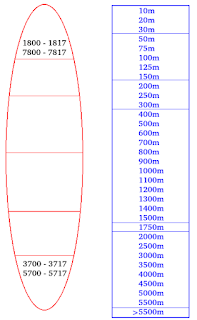
So, notice the graphic at Fig. 1. which has a red oval (surfboard / canoe / paddleboard) shape and a blue rectangle shape which are symbolic of: 1) the shapes of WOD Zones; and 2) the maximum ocean depths in those WOD Zones.
The top cone-shape in the red oval is symbolic of the north polar region (Arctic) and the bottom shape of the red oval is symbolic of the south polar region (Antarctic).
They both (top & bottom) contain numbers which are actual numbers of some of the WOD Zones in them:
Top Cone (layer 0):
1800-1817 = 18 zones in the east (E) longitudes, north (N) latitudes;
7800-7817 = 18 zones in the west (W) longitudes, north (N) latitudes;
(36 zones total).
Bottom Cone (layer 16):
3700-3717 = 18 zones in the east (E) longitudes, south (S) latitudes;
5700-5717 = 18 zones in the west (W) longitudes, south (S) latitudes;
(36 zones total).
The exaggerated red oval shape is curved because the Earth is a globe, which means that the actual zone shapes are not squares.
Since longitude boundaries on a globe are curved, the actual size of the area of the zones diminishes as we move from the equator northward, and from the equator southward.
III. Volume Calculation Considerations
Calculating the area of each zone is the beginning of the exercise (use Haversine Formula and/or Spherical coordinate system):
Zone area = length x width
To complete the calculation & derive the volume, we must multiply the Zone's area by the ocean's depth in that zone, so:
Zone volume = Zone area x Zone depth
The final complication is to 'slice' the total calculated zone volume into thirty-three (33) depth levels shown in the blue rectangle (Fig. 1).
Those 33 depth levels or 'slices' are based on the WOD Manual depths @ Appendix 11 therein.
Since the WOD Manual depths are not uniform (not all the same height/depth, as shown by the blue rectangle) varying in size from 10m to 500m in depth/height, I use a 'percentage multiplier' for each depth level.
In other words, I first calculate the complete volume of the zone, then I derive the volume of each depth-level slice by multiplying the entire volume by a decimal percentage value (e.g. the 10m decimal multiplier is 0.001901141, 20m is 0.003802281, and so forth).
There are 18 layers x 36 zones per layer (648 total Zones) to calculate YIKES! ... oh wait ... some of the Zones are not over the ocean, but over land.
Not to worry, if you use the data sources I mentioned in section 'I' above, they only provide in situ measurements from zones over the oceans (we are observing water, not dirt ☺).
Anyway, the volume calculated is the fixed-mass volume to use without change throughout the next phase.
This critical requirement I just described was also discussed in the previous post (at section 'IV', #1) quoting a peer-reviewed paper (check it out if need be).
IV. Oh yeah, The Measurements
Once we load the in situ values (t=in situ sea water temperature in Celsius, sp = in situ conductivity, aka "salinity", and depth) we can calculate some fundamental TEOS-10 values (using the TEOS-10 C++ version):
z = teosSea.gsw_z_from_p (depth, latitude);Before we move on to calculate thermosteric volume changes (not mass changes) based on sea water temperature changes, we must calculate the thermal expansion coefficient (tec):
p = teosSea.gsw_p_from_z (z, latitude);
sa = teosSea.gsw_sa_from_sp (sp, p, longitude, latitude);
ct = teosSea.gsw_ct_from_t (sa, t, p);
tec = teosSea.gsw_alpha (sa, ct, p)In the following formula, let tvc = thermosteric volume change, mu = mass-unit quantity of depth layer ("ocean slice") mentioned in Section III above, prev_ct = last year's conservative temperature, ct = this year's conservative temperature.
Now we can calculate thermosteric volume change with this formula:
tvc = mu * (1 + (tec * ct - prev_ct))
Since tvc , like mu ("mass-unit", a.k.a. "eustatic"), is in cubic kilometers (km3), to convert tvc into millimeters of thermosteric sea level change (tsSLC), we divide tvc by 361.841 (the number of cubic kilometers per millimeter of ocean water).
V. The Menu
The calculations for thermosteric sea level change worldwide are in graphs linked-to in the following menu of appendices.
The links are to appendices that present all of the WOD zone graphs (36 max) within the specified layer where that zone is located.
The 'All Layers' menu selection links to the mean averages of all the zones in that layer.
| Appendices |
| Layer 0 |
| Layer 1 |
| Layer 2 |
| Layer 3 |
| Layer 4 |
| Layer 5 |
| Layer 6 |
| Layer 7 |
| Layer 8 |
| Layer 9 |
| Layer 10 |
| Layer 11 |
| Layer 12 |
| Layer 13 |
| Layer 14 |
| Layer 15 |
| Layer 16 |
| All Layers |
Each appendix has information about what the graphs reveal about thermal expansion and contraction (via infrared photon movement) for the zone or layer begin graphed.
VI. Closing Comments
I am presenting this post because I updated the SOCCOM data in my SQL database.
I also wanted to review the proper data, formulas, and processes required to properly calculate thermal expansion/contraction of seawater.
This is a public service designed to expose the myth of the bathtub model (The Bathtub Model Doesn't Hold Water, 2, 3, 4, 5).
The next post in this series is here, the previous post in this series is here.
No comments:
Post a Comment