 |
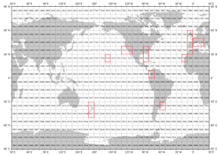
| Fig. 1 Golden 23 Tide Gauge Locations |
I. Introduction
The "Golden 23 Zones" are actually fifteen WOD zones (Fig. 2) which contain the PSMSL "23 golden tide gauge station locations" (Fig. 1) which scientists selected years ago as a valid local-group that is representative of global sea level change (SLC).
The Golden 23 Group's "fingerprints" are also representative of which ice sheets are melting during a given span of time.
The analysis of SLC has been problematic because of, among other things, oversimplification ("Everything should be made as simple as possible, but no simpler." Albert Einstein). and failure to consider or attribute seminal scientific papers (On the robustness of predictions of sea level fingerprints).
 |
| Fig. 2 Golden 23 Zones |
Regular readers know that I was convinced of the use of the golden 23 and have posted about that subject (Golden 23 Zones Revisited).
II. TEOS-10
Since the current dogma concerning SLC is enamored of the notion that SLC is mostly due to thermal expansion, anyone who is seriously looking into that hypothesis, in addition to studying SLC measurement practices, must also take on some of the precepts of oceanography and thermodynamics.
Since I do a lot of research using software modules I construct with C++, I eventually ran across the TEOS-10 toolkit.
It is a special-case toolkit that has the blessings of scientific communities:
The Intergovernmental Oceanographic Commission (IOC), with the(TEOS-10 Flyer, PDF). That EOS-80 usage had led to many an innocent conflicting result over the past 40 years of use.
endorsement of the Scientific Committee on Oceanic Research (SCOR) and the International Association for the Physical Sciences of the Oceans (IAPSO), has adopted the International Thermodynamic Equation Of Seawater - 2010 (TEOS-10) as the official description of seawater and ice properties in marine science. All oceanographers are now urged to use the new TEOS-10 algorithms and variables to report their work.
Fig. 3 Thermosteric Volume
Notable differences of TEOS-10 compared with EOS-80 are :
(1) the use of Absolute Salinity [SA] to describe the salinity of
seawater; Absolute Salinity takes into account the spatially varying composition of seawater. In the open ocean, the use of this new salinity has a non-trivial effect on the horizontal density gradient, and thereby on the ocean velocities calculated via the “thermal wind” relation.
Fig. 4 Absolute Salinity
(2) the use of Conservative Temperature [CT] to replace
potential temperature q. Both of these temperatures are calculated quantities that result from an artificial thought experiment (namely, adiabatic and isohaline change in pressure to the sea surface). Conservative Temperature has the advantage that it better represents the “heat content” of seawater by two orders of magnitude.
Fig. 5 Conservative Temperature
(3) the TEOS-10 properties of seawater are all derived from a
Gibbs function (by mathematical processes such as differentiation) and so are totally consistent with each other (in contrast to the now obsolete EOS-80 approach where separate polynomials were provided for each thermodynamic variable and they were not mutually consistent).
Fig. 6 Sea Pressure
TEOS has led to further improvement as an adjunct to my use of WOD and PSMSL data sets, in terms of analyzing SLC, especially as that analysis involves the hypothesis of thermal expansion induced SLC.
III. The Procedure
Remembering Einstein's guidance about making things as simple as possible, but no more
 |
| Fig. 7 The Volume & Mass Changes |
I query the SQL server for all WOD data from a zone, order it by year, and I also query the SQL server for all PSMSL data from that zone, and also order it by year.
I then pass the WOD data through some TEOS-10 functions to derive the absolute salinity and conservative temperature (the relevant TEOS-10 functions begin with "gsw_").
First, we derive sea pressure from the depth (in meters) that the measurement was taken at (now called "height" in TEOS terminology): p = gsw_p_from_z (depth, latitude); then derive absolute salinity: SA = gsw_sa_from_sp (sp, p, longitude, latitude); and finally derive conservative temperature: ct = gsw_ct_from_t (sa,t,p), where "sp" is the in situ measured salinity that has been recorded in the WOD database, "t" is the in situ measured sea water temperature that has been recorded in the WOD database, and "p" is the sea pressure (dbar) calculated from the measured depth and latitude where the measurements were taken.
 |
| Fig. 8 Sea level rise |
A critical function, in terms of thermal expansion analysis, comes next (the thermal expansion coefficient): tec = gsw_alpha(sa,ct,p), which is required for the final formula which derives thermal volume change (thermal expansion or contraction).
We start with the existing volume of the WOD zone in question.
A bit more "reaching" is required to determine the quantity of sea water (volume or mass) for the ultimate function: ΔV = V0 β ΔT or V1 = V0 * β * (T0 - T1), where V = volume, T = temperature (CT), and β = thermal expansion coefficient.
That is because: 1) the zones are not the same size (as the may seem to be in Fig. 2); 2) they do not have the same depth; 3) they do not have the same amount of land mass (e.g. compare zone 7215 with zone 7308 @ Fig. 2); and 4) not to mention variation in temperature and salinity.
 |
| Fig. 9 TEOS in action |
So, now we can write the TEOS-10 version: zoneV1 = zoneV0 * tec * (CT0 - CT1), where CT0 is last (previous) year and CT1 is this current year, zoneV0 is the zone's beginning volume (prior to the temperature changes in that zone over the year being calculated), and zoneV1 is the new volume after the thermal change calculation has been applied.
The resulting zoneV1 volume can be more (expansion), or less (contraction), than the beginning zoneV0 volume.
These individual zone values are combined to derive the golden 23 mean value.
IV. The Graphs
I use synchronization checks to make sure that the change-patterns match the actual-value-pattern of the entity that is changing in value.
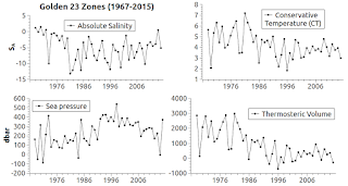
For examples, Fig. 3 checks volume patterns, Fig. 4 checks absolute salinity patterns, Fig. 5 checks conservative temperature patterns, Fig. 6 checks sub-surface water pressure patterns, and Fig. 8 checks SLC patterns.
Those match, so we can now discuss the main feature, while considering the graphs at Fig. 7.and Fig. 9.
V. Calculation
The Fig. 7 ending value for SLC during 1967-2015 is 78.1 mm, and the Fig. 7 ending value for thermosteric volume change is -284.773.
Both expansion and contraction took place, but in the end mass change from the melting of ice sheets and land glaciers was the main feature in this span of time's SLC (assuming I have this TEOS-10 working correctly; I invite comment, criticism, heads-up, etc.).
The critical factor for the thermal expansion hypothesis is global warming impact on the oceans, because, as they say "when water is heated it expands."
In the TEOS-10 world, the Absolute Salinity and Conservative Temperature are the key factors.
As we can see in Fig. 9, those two pillars of the hypothesis fell in value during the time frame we are considering.
This resulted in a small drop in thermosteric volume in the amount of 284.773 cu. km., because as SA and CT go, so goes thermosteric volume.
Nevertheless, sea level measured at golden 23 tide gauge stations registered sea level rise during the same time frame.
VI. Thermal Expansion in The Golden 23 Zones
This does not mean that there was no thermal expansion in other WOD zones, because, among other things, the tide gauge stations are on coast lines.
Another thing is that the highest amounts of sea level rise take place in the deep oceans where ocean mass is increased by not only ice sheet and land glacier melt, but also by relocated ocean mass (The Ghost-Water Constant, 2, 3, 4, 5, 6, 7, 8, 9).
VII. Conclusion
At some point I plan to use the TEOS-10 module, which now seems to be in working order, on all tide gauge stations and all WOD zones combined.
Check out the video below.
Another Dr. Mitrovica video (long version):
08:00 The use of global mean average has led us astray for 100 years.
15:20 Taking the average assumes the imaginary bathtub model.
16:30 It is completely wrong.
21:00 100m of SLF @ Greenland's coast when all ice sheet is gone.
26:40 The Dutch government did not understand the scenario.
28:40 When the ice sheet melts, all the water is distributed in 2 weeks.
29:30 It is error to say that SLF is due only to the land rising.
Short version:


No comments:
Post a Comment