The "powers that be" have corrected some of the errors over the time span of this series, however, the "are we there yet" answer is "not quite".
Currently, one of the more accurate statements is:
"The warming of Earth is primarily due to accumulation of heat-trapping greenhouse gases, and more than 90 percent of this trapped heat is absorbed by the oceans. As this heat is absorbed, ocean temperatures rise and water expands.[1] This thermal expansion contributes to an increase in global sea level. Temperature measurements of the sea surface, taken by ships, satellites and drifting sensors, along with subsurface measurements and observations of global sea-level rise, have shown that the warming of the upper ocean caused sea level to rise due to thermal expansion[2] in the 20th century. Using measurements from Argo profiling floats, we know this warming has continued, causing roughly one-third of the global sea-level rise[3] observed by satellite altimeters since 2004."
(NASA, Understanding Sea Level, underlines and "[]" added). The incorrect or incomplete portions in that statement are underlined and discussed below.
[1] The statement "As this heat is absorbed, ocean temperatures rise and water expands" is only true if the water is above its maximum density (minimum volume). If heat is added to a fresh water volume/mass area that is below 4 deg. C the volume will decrease (thermal contraction), and seawater will do the same when heat is added when its temperature is below its maximum density temperature (see Fig. 1).
[2] The statement "the warming of the upper ocean caused sea level to rise due to thermal expansion" is misleading because sea level is a factor of the entire ocean depth, not just the "upper how-ever-much" of it which that statement may refer to.
[3] The statement "causing roughly one-third of the global sea-level rise" is contrasted by another NASA statement "About half of the measured global sea level rise on Earth is from warming waters and thermal expansion" (NASA JPL).
The most widespread cause of these misunderstandings is the widespread use of improper techniques for comprehending and for calculating thermal expansion and contraction of ocean waters around the globe.
II. Improper/Proper Techniques
One paper I noticed explains a fundamental basis for the proper techniques and procedures involved in proper thermal expansion and contraction analysis of seawater:
"A common practice in sea level research is to analyze separately the variability of the steric and mass components of sea level. However, there are conceptual and practical issues that have sometimes been misinterpreted, leading to erroneous and contradictory conclusions on regional sea level variability. The crucial point to be noted is that the steric component does not account for volume changes but does for volume changes per mass unit (i.e., density changes). This indicates that the steric component only represents actual volume changes when the mass of the considered water body remains constant."
I use the World Ocean Database (WOD) data segmented into thirty three depth levels at several hundred WOD Zones.
Since the WOD Zone boundaries are latitude and longitude determined, and since the Earth is a globe, each WOD Zone's volume and mass varies from zone to zone because the four 'sides' of the zone are different lengths and the ocean depths vary (the zone boundaries appear to be even on the WOD map for easier selection).
But more than that, each separate depth level (L1 - L33) and pelagic group varies (see Section IV below).
So, to comply with the proper way of determining thermal expansion and contraction, one must determine the mass/density of each of the thirty-three depth level segments and calculate them individually.
The next most important factor is called the "Thermal Expansion Coefficient" (TEC) that I calculate using the TEOS-10 function gsw_alpha in the C++ software version:
% gsw_alpha: thermal expansion coefficient with respect to % Conservative Temperature (75-term equation) % % USAGE: % gsw_alpha(SA,CT,p) % % DESCRIPTION: % Calculates the thermal expansion coefficient of seawater with respect to % Conservative Temperature using the computationally-efficient expression % for specific volume in terms of SA, CT and p (Roquet et al., 2015). % % Note that this 75-term equation has been fitted in a restricted range of % parameter space, and is most accurate inside the "oceanographic funnel" % described in McDougall et al. (2003). The GSW library function % "gsw_infunnel (SA,CT,p)" is avaialble to be used if one wants to test if % some of one's data lies outside this "funnel". % % INPUT: % SA = Absolute Salinity [g/kg] % CT = Conservative Temperature (ITS-90) [deg C] % p = sea pressure [dbar] %( i.e. absolute pressure - 10.1325 dbar) % % OUTPUT: % alpha = thermal expansion coefficient [1/K] % with respect to Conservative Temperature % % AUTHOR: % Paul Barker and Trevor McDougall[ help@teos-10.org ] % % VERSION NUMBER: 3.06.12 (25th May, 2020) % % REFERENCES: % IOC, SCOR and IAPSO, 2010: The international thermodynamic equation of % seawater - 2010: Calculation and use of thermodynamic properties. % Intergovernmental Oceanographic Commission, Manuals & Guides # 56, % UNESCO (English), 196 pp. Available from http://www.TEOS-10.org % See Eqn. (2.18.3) of this TEOS-10 manual. % % McDougall, T.J., D.R. Jackett, D.G. Wright and R. Feistel, 2003: % Accurate and computationally efficient algorithms for potential % temperature and density of seawater. J. Atmosph. Ocean. Tech., 20, % pp. 730-741. % % Roquet, F., G. Madec, T.J. McDougall, P.M. Barker, 2015: Accurate % polynomial expressions for the density and specifc volume of seawater % using the TEOS-10 standard. Ocean Modelling., 90, pp. 29-43. % % The software is available from http://www.TEOS-10.org % % double TeosBase::gsw_alpha(double sa, double ct, double p) {
/** for GSW_TEOS10_CONSTANTS use gtc */ double xs, ys, z, v_ct_part;
(gsw_alphain the C++ version of source code library). I don't know if this function is available in the other software versions.
Finally, all of the above procedures (Section II) must be done in a proper sequence as follows:
1) use the same exact data used to calculate potential enthalpy used in Dredd Blog post The Photon Current - 10.
2) use the same exact TEOS-10 functions that were used in that post to generate Conservative Temperature (CT), Absolute Salinity (SA), and pressure (P).
3) then use the gsw_alpha function to generate the TEC; then this formula to generate the thermal expansion/contraction value:
V1 = V0 * (1.0 + (B * DT))
where:
V0 = mass_unit_vol
DT = D - T
D = current temperature B = thermal expansion/contraction coefficient (TEC); T = previous temperature V1 = thermal expansion/contraction (volume change)
Sorry if I have oversimplified this discussion.
III. Appendix Details
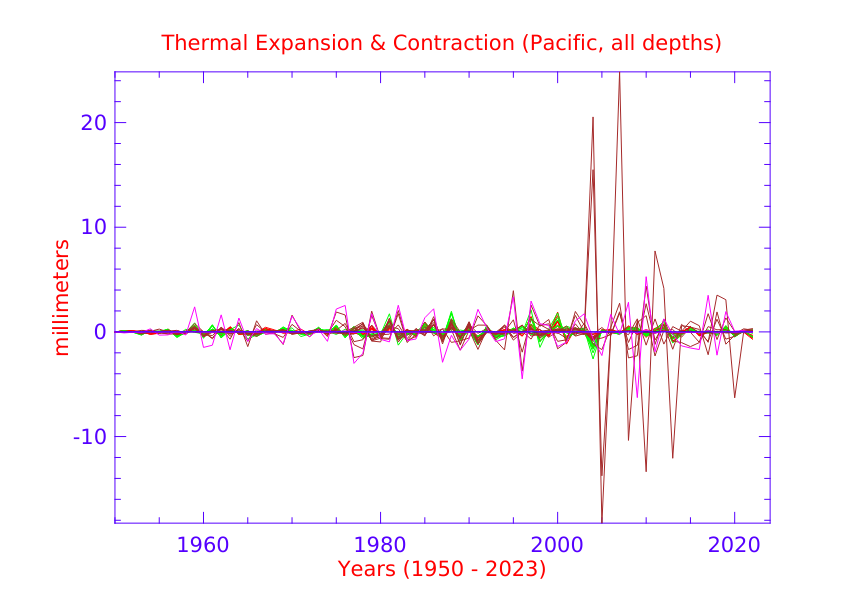
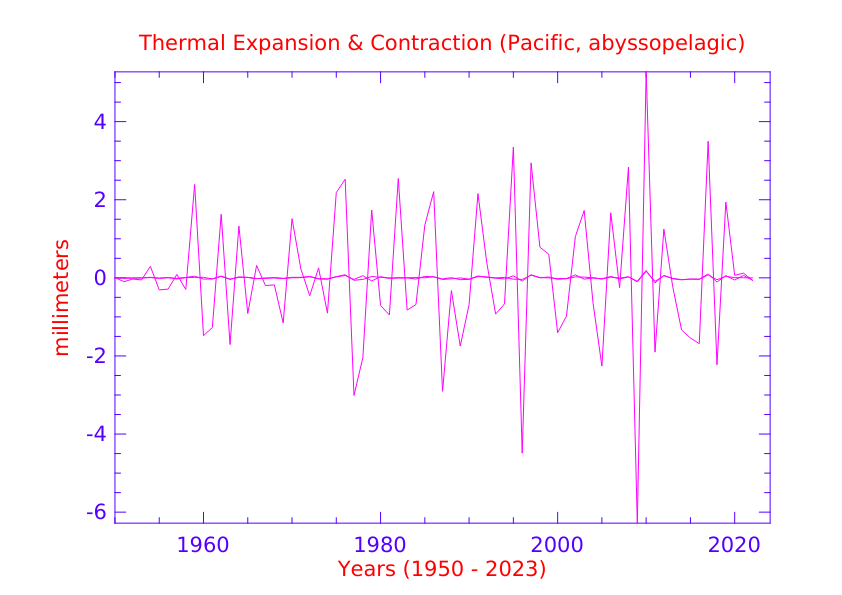
The main ocean areas involved are the Arctic, Southern, Atlantic, Indian, and Pacific.
In addition, three 'ocean groups' (smaller ocean areas combined together) are featured, which are composites as follows:
Group Misc_1 is composed of data from Mediterranean, Black_Sea, Baltic_Sea, Persian_Gulf, Red_Sea, Sulu_Sea and Yellow_Sea sources.
Group Misc_2 is composed of data from Sea_of_Japan, Seto_Inland_Sea, Hudson_Bay, Andaman_Sea, Arabian_Sea, Bay_of_Bengal, and Bering_Sea sources.
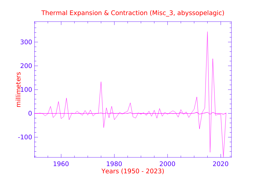
Group Misc_3 is composed of data from Caribbean_Sea, Gulf_of_Mexico, North_Sea, South_China_Sea, Sea_of_Okhotsk, and Adriatic_Sea sources.
Today's appendices are another viewpoint of the same exact WOD in situ data featured in The Photon Current - 10, but the appendices in that post dealt with "potential enthalpy" a.k.a. "photons of ocean heat" while today's appendices deal with thermal expansion and contraction at the same ocean areas (Appendix 1, Appendix 2, Appendix 3, Appendix 4, Appendix 5, Appendix 6).
VI. Closing Comments
The averages are calculated by initially using the temperature, salinity, and depth values (the in situ measurements of the WOD database) by zone, year, and depth.
Those values are then averaged in an array, and finally blanks between years and depth values are filled in by averaging.
The purpose of this post is to give a general idea of what is missing when only the upper ~2,000 meters of the oceans are used to estimate thermal expansion.
Infrared photons carrying ocean heat from warm seawater to cooler seawater do not stop at the 2,000 meter or any other "upper ocean" depth boundary.
Instead, over time those photons obeying the Second Law of Thermodynamics go all the way to the seafloor:
"[Classical Thermodynamics] is the only physical theory of universal content which I am convinced will never be overthrown, within the framework of applicability of its basic concepts."
The full results of thermal expansion and thermal contraction is as follows:
Atlantic (Per annum net thermosteric change: 0.0470611 mm)
Pacific (Per annum net thermosteric change: 0.00319018 mm)
Indian (Per annum net thermosteric change: 0.779715 mm)
Southern (Per annum net thermosteric change: 0.0154316 mm)
Arctic (Per annum net thermosteric change: 0.0412511 mm)
Misc_1 (Per annum per group member net thermosteric change: 0.0597841 mm)
Misc_2 (Per annum per group member net thermosteric change: 0.111403 mm)
Misc_3 (Per annum per group member net thermosteric change: 0.174235 mm)
These values in millimeters are the bottom line average thermosteric changes per year.
These values were derived by adding the thermal expansion (positive numbers) and thermal contraction (negative numbers) together for each depth level in each ocean area WOD Zone and each ocean group, then dividing that sum by the number of years involved.