Pages

Saturday, October 6, 2018

On Thermal Expansion & Thermal Contraction - 38

Fig. 1 WOD Layers (0-17)
I have finished a module that does precision sea level change calculations using all of the WOD datasets that contain both temperature (T) and salinity (SP) measurements (XBT and MBT are excluded).

This module works on WOD layers as shown by the graphic at Fig. 1.

Some results, in terms of mean average, are shown on the graph at Fig. 2 (just so you know, the ending sea level rise values show that thermal expansion was 2.37% of the total sea level rise).
Fig. 2 Sea level change

Thermal expansion was 2.62688 mm, while total sea level rise as measured at tide gauge stations around the globe was 110.855 mm (the percentage arithmetic is: 2.62688 ÷ 110.855 = 0.023696541 = 2.37%).

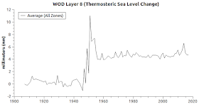
The graphs at Fig. 3 - Fig. 19 detail the mean average of each WOD layer's thermal expansion & contraction at each Zone in each layer (Fig. 1 shows the zones in each layer).

I had never graphed those measured values going that far back (1800's) before, because the WOD CTD and PFL datasets I used did not go back past the 1960's.

I began to use all WOD Datasets a while back, so the 1800's can now be done (Databases Galore - 22, 23, 24, and 25).

Fig. 3 Layer 0
Fig. 4 Layer 1
Fig. 5 Layer 2
Fig. 6 Layer 3
Fig. 7 Layer 4
Fig. 8 Layer 5
Fig. 9 Layer 6
Fig. 10 Layer 7
Fig. 11 Layer 8
Fig. 12 Layer 9
Fig. 13 Layer 10
Fig. 14 Layer 11
Fig. 15 Layer 12
Fig. 16 Layer 13
Fig. 17 Layer 14
Fig. 18 Layer 15
Fig. 19 Layer 16
I did try to calculate and estimate seawater temperatures backwards into the 1800's, based on the GISS atmospheric temperature changes, by transferring about 93% of the atmospheric changes into the ocean temperatures over that time frame.

Since the GISS atmospheric temperature declines as one goes back in time, so did my estimation of ocean temperatures.

The measured values we now have do not follow that computed pattern.

Compare "On Thermal Expansion & Thermal Contraction - 19", at Fig. 2 therein, with "On Thermal Expansion & Thermal Contraction - 37", at Fig. 3c therein.

The older measurements defied my declining temperature expectations and logic as to past temperatures.

As we go back in time far enough the measurements made then were probably not taken at some of the locations they are routinely taken at now (e.g. ARGO floats).

Nor were measurements taken at deep-depths where water in non-polar zones is generally cooler.

Wooden sailing ships and even coal fired steamers had limited ocean access due to weather conditions and traveling time required.

Fuel, food, fresh water, and other supplies only lasted so long.

So, either there were technical difficulties with gathering data in extreme or far away places, or the ocean temperature trends then are contrary to our more recent observations and measurements of trends.

I doubt the latter ("ocean was different then"), because sea level change, as measured by tide gauge stations going back to the 1700's, indicates that warming has increased since the late 1700's because melting has increased since then (Proof of Concept, 2, 3, 4, 5, 6, 7, 8, 9).

The GISS atmospheric temperature measurements at weather stations around the globe also indicate that atmospheric warming has increased just a bit over 1 degree C over that time frame.

How SLC Graphs Are Made

Today's graphs are about thermosteric sea level change.

That is, change brought about by changing ocean temperatures.

The mean average sea level change shown in Fig. 2 was calculated using all PSMSL tide gauge station records and all WOD dataset measurements containing both T (temperature) and SP (salinity) values.

The XBT and MBT datasets are excluded from this exercise.

They do not contain any SP measurements with which to match the T measurements and thereby do TEOS calculations.

Anyway, the procedure is to gather the measurements into an array based on sequential years from 1800 to the present.

That means using values measured from up to 33 depth level sections or slices of varying sizes (10m, 20m, 30m, 50m, 75m, 100m, 125m, 150m, 200m, 250m, 300m, 400m, 500m, 600m, 700m, 800m, 900m, 1000m, 1100m, 1200m, 1300m, 1400m, 1500m, 1750m, 2000m, 2500m, 3000m, 3500m, 4000m, 4500m, 5000m, 5500m, and >5500m).

Note that when calculating thermal expansion both mass-unit (how many molecules) and volume (distance between molecules) must be taken into consideration.

The formula "volume = length times width times height" (v = l * w * h) must be used to calculate individual depth level mass-units because "h" is different at some depth levels.

For example h=10 at depth-level 0 to 10m, but h=500 at depth-level 3500m to 4000m.

Thus, a volume calculation for each of the depth-level mass-units must take place when one is calculating their individual thermal expansion / contraction values.

Not only that, WOD zones themselves have different "w" values because longitude width varies (progressively narrower moving from the equator toward the poles, and vice versa pole to equator).

So, each "cubic" section (depth-level mass-unit) of each zone is calculated independently for volume change caused by temperature change (thermal expansion / contraction).

The process goes like this for each WOD zone and each depth level:

1) calculate the mass-unit of the zone's water column depth level (v=l*w*h);

2) convert T and SP values into TEOS-10 Conservative Temperature (CT) and Absolute Salinity (SA) values;

3) calculate the thermal expansion coefficient (tec) using the TEOS-10 gsw_alpha function;

4) calculate the change in temperature at each depth-level mass-unit from one year to the next (an increase in temperature will generally mean thermal expansion while a decrease in temperature will generally mean thermal contraction);

5) derive the net change in volume ("vc") (not the mass-unit "mu") for each zone at each depth-level:
vc = mu * (1 + ( tec * ct - prev_ct ))
6) sum the volume change ("vc") increases and decreases at each depth-level of each zone;

7) to derive a mean average for that layer, sum the "vc" zone changes for each WOD latitude layer, then divide that sum by the number (count) of "vc" values in that latitude layer.

The initial mass-unit ("mu") of each depth level must remain constant throughout the span of years of the calculations, because the thermosteric volume changes (increases and decreases) are the "vc" ... not the "mu" (mass-unit).

The "vc" is what changes from year to year due to thermal changes.

It is important that the "mu" ("l" * "w" * "h") value for each mass-unit (depth-level water quantity) in each zone must not change while doing the thermosteric calculations (note the "l,w,h" example mass-unit for Bathypelagic depth-level @ Fig. 20):
Fig. 20 Bathypelagic mass-unit
"A common practice in sea level research is to analyze separately the variability of the steric and mass components of sea level. However, there are conceptual and practical issues that have sometimes been misinterpreted, leading to erroneous and contradictory conclusions on regional sea level variability. The crucial point to be noted is that the steric component does not account for volume changes but does for volume changes per mass unit (i.e., density changes). This indicates that the steric component only represents actual volume changes when the mass of the considered water body remains constant."
(Journal of Geophysical Research: Oceans, emphasis added). Once the proper techniques are in place, the process is straightforward.

The next post in this series is here, the previous post in this series is here.


Wednesday, October 3, 2018

Make Steroids Great Again

New York B4 The Steroids
Whales After The Steroids
One of the most popular Dredd Blog posts is about plastics (New Continent Found - Garbage Gyre II).

That Dredd Blog post caused a stir among young Catholics, the Kavanaughts, who live in heaven instead of here on Earth alongside us mortals (You Are Here).

Anyway, one American with vision to spare puts it this way:
"When you think about it, Earth is a relatively modest-sized planet -- about 25,000 miles in circumference at the Equator, with a total surface area of 197 million square miles, almost three-quarters of which is water. It’s not so hard, if you’re in a certain frame of mind (as American officials were after 1991), to imagine that a single truly great nation -- a “sole superpower” with a high-tech military, its capabilities unparalleled in history -- might in some fashion control it all.

Think back to that year when the other superpower, the lesser one of that era, so unbelievably went down for the count. Try to recall that moment when the Soviet Union, its economy imploding, suddenly was no more, its various imperial parts -- from Eastern Europe to Central Asia -- having largely spun free. It’s hard now to remember just how those months after the fall of the Berlin Wall in 1989 and that final moment in 1991 stunned the Washington establishment. Untold sums of money had been poured into “intelligence” during the almost half-century of what became known as the Cold War (because a hot war between two nuclear-armed superpowers seemed unimaginable -- even if it almost happened). Nonetheless, key figures in Washington were remarkably unprepared for it all to end. They were stunned. It simply hadn’t occurred to them that the global standoff between the last two great powers on this planet could or would ever truly be over.

And when you think about it, that wasn’t so illogical. Imperial rivalries had been the name of the game for so many centuries. A world without some version of such rivalries seemed genuinely unimaginable -- until, of course, it happened. After the shock began to wear off, what followed was triumphalism of a soaring sort. Think of that moment as the geopolitical equivalent of a drug high."
(In the Heart of a Dying Empire, Tom Dispatch). The Kavanaughts are now here to make America grunt again (How To Identify The Despotic Minority).

Another American with vision to spare puts it this way:
"So, of all Trump’s policies, the one that is the most dangerous and destructive, in fact poses an existential threat, is his policies on climate change, on global warming. That’s really destructive. And we’re facing an imminent threat, not far removed, of enormous damage. The effects are already visible but nothing like what’s going to come. A sea level rise of a couple of feet will be massively destructive. It will make today’s immigration issues look like trivialities. And it’s not that the administration is unaware of this. So, Donald Trump, for example, is perfectly aware of the dangerous effects, in the short term, of global warming. So, for example, recently he applied to the government of Ireland for permission to build a wall to protect his golf course in Ireland from rising sea levels. And Rex Tillerson, who was supposed to be the adult in the room before he was thrown out, as CEO of ExxonMobil, was devoting enormous resources to climate change denial, although he had, sitting on his desk, the reports of ExxonMobil scientists, who, since the '70s, in fact, were on the forefront of warning of the dire effects of this accelerating phenomenon. I don't know what word in the language—I can’t find one—that applies to people of that kind, who are willing to sacrifice the literal—the existence of organized human life, not in the distant future, so they can put a few more dollars in highly overstuffed pockets. The word “evil” doesn’t begin to approach it. These are the kinds of issues that should be under discussion. Instead, what’s being—there is a focus on what I believe are marginalia."
(Chomsky, emphasis added) "Marginalia" (of current civilization) is an idea that gives new meaning to "lost civilizations."


Willie Nelson:


Pete Seeger:


Bob Dylan:


On Thermal Expansion & Thermal Contraction - 37

Fig. 1 Thermosterics
The WOD Datasets (Databases Galore - 25) that I am now working with have characteristics (in a couple of them) that thwart the calculation of thermal expansion and other characteristics of seawater.

I mean direct calculation by way of in situ measurements of both temperature and conductivity (salinity).

That is because only temperature is recorded in them.

I am talking about the MBT and XBT datasets.

The TEOS-10 functions for calculating thermal expansion require both T (temperature) and SP (practical salinity ... or conductivity) in order to calculate thermal expansion.

The process goes like this: 1) collect the temperature "T" and "SP" (conductivity) at depth "D"; 2) convert SP into Absolute Salinity (gsw_SA_from_SP); and 3) convert "T" into "CT" (gsw_CT_from_t).

That part is quite straightforward, unless of course "SP" is missing, as pointed out in TEOS-10 publications:
"3. Absolute Salinity SA

Perhaps the most apparent change in using TEOS-­‐‐10 compared with using the International Equation of State of seawater (EOS-­‐‐80) is the adoption of Absolute Salinity SA instead of Practical Salinity SP (PSS-­‐‐78) as the salinity argument for evaluating the thermodynamic properties of seawater. Importantly, Practical Salinity is retained as the salinity variable that is stored in national databases. This is done to maintain continuity in the archived salinity variable, and also because Practical Salinity is virtually the measured variable (whereas Absolute Salinity is a calculated variable).

The “raw” physical oceanographic data, as collected from ships and from autonomous platforms (e. g. Argo), and as stored in national oceanographic data bases, are
• Practical Salinity (SP , unitless, PSS-­‐‐78) and
• in situ temperature (t, °C , ITS-­‐‐90) as functions of
• sea pressure ( p, dbar ), at a series of
• longitudes and latitudes.
Under TEOS-­‐‐10 all the thermodynamic properties are functions of Absolute Salinity SA (rather than of Practical Salinity), hence the first step in processing oceanographic data is to calculate Absolute Salinity, and this is accomplished by the GSW function gsw_SA_from_SP. Hence the function gsw_SA_from_SP is perhaps the most fundamental of the GSW functions as it is the gateway leading from oceanographic measurements to all the thermodynamic properties of seawater under TEOS-­‐‐10. A call to this function can be avoided only if one is willing to ignore the influence of the spatial variations in the composition of seawater on seawater properties ..."
(Getting Started, TEOS-10, PDF). The unique expansion/contraction properties (Fig. 1) of both pure water and seawater can't be fully discerned without an evaluation of Absolute Salinity (SA).
Fig. 2a MBT Dataset
Fig. 2b XBT Dataset

This series has considered that reality from several viewpoints (On Thermal Expansion & Thermal Contraction, 2, 3, 4, 5, 6, 7, 8, 9, 10, 11, 12, 13, 14, 15, 16, 17, 18, 19, 20, 21, 22, 23, 24, 25, 26, 27, 28, 29, 30, 31, 32, 33, 34, 35, 36).

Nevertheless, today I have displayed the two datasets (MBT, XBT) which contain only "T" (excluding "SP") measurements just to show readers that I do have that data (Fig. 2a - Fig. 2b).

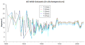
I have also furnished a mean average graph of all "T" measurements in the WOD Datasets (Fig. 3c); a comparison of mean average "T" values to MBT measurements of "T" (Fig. 3a); and finally the same comparison with respect to XBT (Fig. 3b).

Fig. 3a Mean Average (during MBT years)
Fig. 3b Mean Average (during XBT years)
Fig. 3c Mean Average of "T" (all years)
You can see, by those comparisons, that the MBT and XBT datasets are limited both in terms of span of time as well as being devoid of salinity (SP) measurements.

That is why they were not contained in previous graphs of the WOD Datasets that displayed Conservative Temperature (CT) and Absolute Salinity (SA) values.

So, let me move on to further elaborate why this is of fundamental importance.

I have complained often about the mythic mantra that "thermal expansion is the main cause of sea level rise over the past century" as follows:
"Thermal expansion of pure water does not have the same thermodynamic events that the thermal expansion of sea water has.

Nevertheless, you can search the Internet and find videos of someone pouring pure water into a flask, making a mark on the flask, then heating the flask with a Bunsen Burner.

Then, after the water warms, they will put another mark on the flask ostensibly showing that the heat has caused the water to increase in volume.

Then they are apt to declare that this proves that thermal expansion is the major cause of sea level rise because "as water warms it expands."

The problem with this Mickey Mouse trick is that the pure water they use is at a temperature that is not below its maximum density temperature of 4 deg. C when they apply heat to the flask."
(On Thermal Expansion & Thermal Contraction - 36). Using drinking water to argue elements of seawater behavior is moronic.

I have detailed how to build your own system, using the most advanced thermodynamic tools available (Build Your Own Thermosteric Computational System).

In closing, let me include the critical TEOS-10 functions when one is contemplating the calculation of thermosteric volume change in seawater (i.e. thermal expansion / contraction):
"Once we load the in situ values (t=in situ sea water temperature in Celsius, sp = in situ conductivity ("salinity"), and depth) we can calculate some fundamental TEOS-10 values.
z = gsw_z_from_p (depth, lat);
p = gsw_p_from_z (z, lat);
sa = gsw_sa_from_sp (sp, p, lon, lat);
ct = gsw_ct_from_t (sa, t, p);
ctmd = gsw_ct_maxdensity (sa, p);
Before we move on to calculate thermosteric volume changes (not mass changes) based on sea water temperature changes, we must calculate the thermal expansion coefficient (tec):
tec = gsw_alpha (sa, ct, p)
In the following formula, let vc = volume change, vol = mass-unit volume of depth layer ("ocean slice") mentioned in Section III above, prev_ct = last year's conservative temperature, ct = this year's conservative temperature.

Now we can calculate thermosteric volume change with this formula:
vc = vol * (1 + (tec * ct - prev_ct))
Since vc , like vol, is in cubic kilometers (km3), to convert vc into millimeters of sea level change (SLC), we divide vc by 361.841, which is the number of cubic kilometers per millimeter of SLC."
(ibid, Build Your Own Thermosteric Computational System). I will be generating thermal expansion / contraction graphs from the 1800's using all the WOD Datasets (except MBT and XBT) to the present in upcoming posts.

(Although, I may first get into some cultural phenomena posts seeing as how the USA is degenerating as fast as, or perhaps faster than, the Cryosphere.)

The next post in this series is here, the previous post in this series is here.

Monday, October 1, 2018

Databases Galore - 25

Fig. 1a Mean Average (CT)
Fig. 1b Mean Average (SA)
I. Some Background

Regular readers know that, as far as deep-ocean characteristics, in the past I typically used only two WOD Datasets (CTD and PFL)  until recently (Databases Galore - 2223, and 24).

Today, I want to complete the narrative and the description of that change in Dredd Blog sources.

To do explain more about the specific characteristics of the data I will quote from the World Ocean Database Manual (PDF).

I am also using some long term (c. 1860 - 2018) graphs which present the data from those individual datasets in their collective (mean average) format as well as showing them along side each other in their individual format.

The technical format is TEOS-10 (in situ graphs were previously displayed here).

But before I get into the variations on the theme, let me mention Fig. 1a and Fig. 1b.

Those graphs show Conservative Temperature (CT) and Absolute Salinity (SA) during the span of time (1950 - 2018) when instruments used to measure seawater characteristics have been "improved versions."
Fig. 2a Mean Average (CT)
Fig. 2b Mean Average (SA)

II. Historical Variety

The complete span-of-time graphs of the same CT and SA, which include in situ measurements collected by scientists using less sophisticated instruments in times past.

The graphs depicting that, as well as data collected while using the most recent and most sophisticated instruments for collecting such measurements, are shown at Fig. 2a and Fig. 2b.

III. Data Collection Variety

 The variation in results gathered over time is not difficult to discern, nor is it difficult to discern the variation in results caused by using a variety of instruments and a variety of collection techniques.

The graphs at Fig. 3a through Fig. 5b are paired CT & SA depictions of the datasets without the mean average values in graphs Fig. 2a and Fig. 2b.

Those graphs illustrate the significant differences in measurement varieties in the datasets.

IV. Dataset Descriptions in the WOD Manual

The following descriptions (between the two lines) are quoted from the manual (WORLD OCEAN DATABASE 2013 USER’S MANUAL, June 28, 2016, Version 2.2, pp. 5-7, pp. 15-17 PDF).

Note: the graphs are not in the manual.

D. DATASETS
The data in WOD13 are organized into eleven datasets that are briefly described in this section and listed in Table 2. A more detailed explanation of each dataset is provided in individual chapters of the World Ocean Database 2013 NOAA Atlas NESDIS 72 (Boyer et al., 2013).

1. Ocean Station Data (OSD)
Historically, Ocean Station Data (OSD) referred to measurements made from a stationary research ship using reversing thermometers to measure temperature and making measurements of other variables such as salinity, oxygen, nutrients, chlorophyll, etc. on seawater samples gathered using special bottles. The OSD dataset includes bottle data, low-resolution Conductivity-Temperature-Depth (CTD) data, Salinity- Temperature- Depth (STD), some surface-only data with specific characteristics, some low-resolution Expendable XCTDs, and plankton taxonomic and biomass measurements.

2. High-Resolution Conductivity-Temperature-Depth (CTD) Data
The CTD dataset contains data from Conductivity-Temperature-Depth instruments as well as STD data measured at high frequency vs. depth (pressure). CTD data are treated according to their resolution. All casts with a depth increment less than two meters are considered high-resolution CTD otherwise, the casts are considered as low-resolution CTD. The low-resolution CTD data reside within OSD dataset. High-resolution data collected by expendable Conductivity-Temperature-Depth (XCTD) instruments are also included in this dataset.

Fig. 3a CT (10m)
Fig. 3b SA (10m)
Fig. 4a CT (100m)
Fig. 4b SA (100m)
Fig. 5a CT (800m)
Fig. 5b SA (800m)
3. Mechanical/Digital/Micro Bathythermograph (MBT) Data
The MBT instrument was developed in its modern form around 1938 (Spilhaus, 1938). The instrument provides estimates of temperature as a function of depth in the upper water column. The MBT dataset contains data on water temperature profiles obtained from MBTs, Digital Bathythermograph (DBT) and Micro Bathythermograph (micro BT) instruments.

4. Expendable Bathythermograph (XBT) Data
The XBT was first deployed around 1966 and replaced the MBT in most measurement programs. This electronic instrument has a thermistor which measures temperature vs. depth. Depth is calculated using the elapsed time of its free descent through the water column and fall-rate equation. (See Section IV for information on XBT fall-rate error.)

5. Surface (SUR) Only Data
The SUR dataset contains data collected by any in-situ means from the surface of the ocean. The majority of the SUR observations were performed along ship routes in the Atlantic and Pacific oceans. In the SUR dataset each cruise is stored in the same form as a cast for other datasets. Each measurement has an associated latitude, longitude, and Julian year-day.

6. Autonomous Pinniped (APB) Data
The APB dataset contains in-situ temperature data from time-temperature-depth recorders (TTDR) and temperature and salinity data from CTD sensors manually attached to marine mammals such as northern elephant seals (Mirounga angustirostris).

7. Moored Buoy (MRB) Data
The MRB dataset contains temperature and salinity measurements collected from moored buoys located in the Tropical Pacific, tropical Atlantic, Baltic and North Seas, and area around Japan. These include the major ongoing Equatorial buoy arrays, TAO/TRITON, PIRATA, and RAMA.

8. Profiling Float (PFL) Data
The PFL dataset contains temperature and salinity data collected from drifting profiling floats such as Profiling Autonomous Lagrangian Circulation Explorer (P-ALACE), PROVOR (free-drifting hydrographic profiler), SOLO (Sounding Oceanographic Lagrangian Observer), and APEX (Autonomous Profiling Explorer). The main source of the PFL data in WOD13 is the Argo project.

9. Drifting Buoy (DRB) Data
The DRB dataset contains data collected from surface drifting buoys and drifting floats with subsurface thermister chains. The major sources of this data include the GTSPP project and Arctic buoy projects.

10. Undulating Oceanographic Recorder (UOR)
The UOR dataset contains data collected from a ConductivityTemperature-Depth probe mounted on a towed undulating vehicle. A description of the different types of UOR vehicles used for acquiring the data included in the WOD13 can be found in Appendix 2.21.

11. Glider (GLD) Data
The GLD dataset contains data collected from reusable autonomous underwater vehicles (AUV) designed to glide from the ocean surface to a programmed depth and back while measuring temperature, salinity, depth-averaged current, and other quantities along a sawtoothed trajectory through the water.


V. Conclusion

As the graphs in Section IV above show, the data variety is obvious.

What causes the variety is not so obvious.

Many things can play a part in the variety, that is why mean average in this context is less of a problem than it is in sea level change scenarios.

The previous post in this series is here.