Dredd Blog: 2021-10-10

Ye olde in situ tracks
and new Quantum Tracks

I. Introduction

Today's Dredd Blog post concerns, among other things:

1) a "dot org (.org)" which Wikipedia describes as: "NWO funds ... and steers the course of Dutch science by means of subsidies and research programmes" (Wikipedia);

2) a paper funded by that "dot org (.org)" (Exploring Sources of Uncertainty in Steric Sea-Level Change Estimates).

Going forward, that paper will be called the 'NWO Paper' in this post.

Additionally, I will introduce the "Sizemograph Algorithm" software which, like the Seismograph, writes graphs of movements.

The Earthquake Glossary describes a Seismograph as an "A seismograph, or seismometer, is an instrument used to detect and record earthquakes."

Dredd Blog describes the "Sizemograph Algorithm" (Sizemograph) as "software that makes a Seismograph-like record of thermosteric changes in ocean water volume at up to thirty-three depth levels."

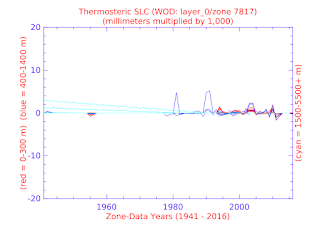
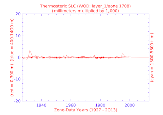
The appendices to today's Dredd Blog post display the graphic results of the Sizemograph using in situ measurements from World Ocean Database (WOD) zones (you can acquire those ~5.5 billion WOD in situ measurements cost-free here).

II. Funding

The 'art' of funding has steered the research world's direction since dirt was first discovered, nevertheless, when the 'truth is found to be lies', there remains independent research that leads to actual discovery (The Warming Science Commentariat - 12).

III. History Writ Large

Once upon a time there was Newtonian Mechanics to help steer Oceanography, but now that has been enhanced in many ways by Quantum Mechanics.

Quantum Oceanography is the quantum mechanics version of a portion of Oceanography which now researches seawater dynamics using photon reality.

IV. The Basics (Classics)

The NWO Paper's 'Abstract' points out what it seeks to accomplish as:

"Recent studies disagree about the contribution of variations in temperature and salinity of the oceans—steric change—to the observed sea‐level change. This article explores two sources of uncertainty to both global mean and regional steric sea‐level trends."

(NWO Paper). That disagreement is not a recent problem, so "recent studies" is not sufficiently comprehensive IMO.

For years Dredd Blog has cited scientific papers that specifically point out the two major calculation-specific reasons, and the one major data usage reason (three reasons total) for why "studies disagree" on thermal expansion dynamics.

Concerning the two major calculation-specific reasons:

(1) "A common practice in sea level research is to analyze separately the variability of the steric and mass components of sea level. However, there are conceptual and practical issues that have sometimes been misinterpreted, leading to erroneous and contradictory conclusions on regional sea level variability. The crucial point to be noted is that the steric component does not account for volume changes but does for volume changes per mass unit (i.e., density changes). This indicates that the steric component only represents actual volume changes when the mass of the considered water body remains constant."

(quoted in: On The More Robust Sea Level Computation Techniques).

(2) "The quest in this work is to derive a variable that is conservative, independent of adiabatic changes in pressure, and whose conservation equation is the oceanic version of the first law of thermodynamics. That is, we seek a variable whose advection and diffusion can be interpreted as the advection and diffusion of ‘heat.’In other words, we seek to answer the question, ‘what is heat’ in the ocean?

...
The variable that is currently used for this purpose in ocean models is potential temperature referenced to the sea surface, θ, but it does not accurately represent the conservation of heat because of (i) the variation of specific heat with salinity and (ii) the dependence of the total differential of enthalpy on variations of salinity.
...
For example, an increase in pressure of 10⁷ Pa (1000 dbar), without exchange of heat or salt, causes a change in enthalpy that is equivalent to about 2.5ЊC. We show in this paper that in contrast to enthalpy, potential enthalpy does have the desired properties to embody the meaning of the first law.
...
Present treatment of oceanic heat fluxes is clearly inconsistent. Ocean models treat potential temperature as a conservative variable and calculate the heat flux across oceanic sections using a constant value of heat capacity. By contrast, heat flux through sections of observed data is often calculated using a variable specific heat multiplying the flux of potential temperature per unit area (Bryan 1962; Macdonald et al. 1994; Saunders 1995; Bacon and Fofonoff 1996). Here it is shown that the theoretical justification of this second approach is flawed on three counts. While the errors involved are small, it is clearly less than satisfactory to have conflicting practices in the observational and modeling parts of physical oceanography, particularly as an accurate and convenient solution can be found.
...
it is perfectly valid to talk of potential enthalpy, h⁰, as the 'heat content' ...”

(quoted in: In Search Of Ocean Heat).

Concerning the major data specific reason:

(3) "Using a plastic water bottle, food coloring, a straw, and a ruler, Connor was able to measure the water rising inside the water bottle. By shining a heat lamp on the water bottle, he was able to track the water’s height as time went on. After 45 minutes, the temperature rose from 72 degrees Fahrenheit to 113 degrees Fahrenheit causing the water to rise seven centimeters. This experiment clearly showed how the thermal expansion of water can lead to rising sea levels."

(quoted in: On Thermal Expansion & Thermal Contraction - 42).

NOTE: That experiment only contains one depth level, whereas the ocean has many depth levels.

The NWO Paper makes those same three basic mistakes, in that:

1) it does not differentiate the mass values of the ocean depth area being considered and thereby does not distinguish the mass of the ocean depth level slice as a fixed mass;

2) it does not calculate using potential enthalpy, instead using potential temperature, as a consequence of using current ocean models; and

3) it does not use in situ measurements from all ocean depths ("We limit our analysis to the upper ocean (0–2,000 m)") which they admit is problematic ("the deep ocean (>2,000 m depth) contribution to steric SLC is uncertain. Given the lack of observational data below 2,000 m depth"). The NWO Paper did not choose to use the WOD datasets for those depths (see NWO paper at Table 1), so they can't complain that there are not enough in situ measurements to go below 2000m and instead just leave it "for future work" (ibid).

Yet, the NWO Paper claims to be able to more accurately calculate/estimate/guesstimate all the uncertainty it considered.

V. The Quantification (Quantum Oceanography)

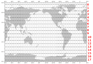
WOD Layers & Zones

As in the Dredd Blog post that took a look at ocean surface to bottom in a thirty-three (33) depth level scenario, today's Sizemograph reports are similar in that sense.

The appendices below show the volatility of thermosteric sea level change when the Sizemograph does its work all the way to the ~~bone~~ bottom:

Appendices

The Sizemograph works substantially the same way as the Conservative Temperature (CT) graph maker did in the previous post.

The difference is that the Sizemograph makes graphs of Thermosteric Sea Level Change (TSSLC) instead of graphing CT.

VI. Closing Comments

The NWO Paper is in error when it claims, inter alia, that the use of 'noise' is the better way to determine why inconsistencies exist.

For additional reading on the subject in general see e.g. On Thermal Expansion & Thermal Contraction, 2, 3, 4, 5, 6, 7, 8, 9, 10, 11, 12, 13, 14, 15, 16, 17, 18, 19, 20, 21, 22, 23, 24, 25, 26, 27, 28, 29, 30, 31, 32, 33, 34, 35, 36, 37, 38, 39, 40, 41, 42.

You are welcome.

The Cryosphere realm to intelligently focus on is the grounding line of tidewater glaciers in Antarctica and Greenland (The Ghost Plumes - 13; Antarctica 2.0 - 11).

Any Questions?

The next post in this series is here, the previous post in this series is here.

Ode to the shallow water skimmers: