|
| Fig. 1 |
As a follow-up to
the previous post in this series, I wanted to share some facts about the data I use to generate graphs that regular readers peruse.
I want you to know that a lot of work goes into it, but sometimes it may not show.
Database management, such as the
World Ocean Database (WOD) and the
Permanent Service for Mean Sea Level (PSMSL) are as much a part of modern science as looking through a microscope is.
Especially in the sense that they make the data available to us for our close scrutiny, to help us discern the junk from the science.
Looking back on
Labor Day, I wanted you to have a better understanding of why I criticize those who want to take the work out of science, by taking the data gathering and sharing out of it.
In today's post, I will also show some appreciation for the scientists who painstakingly gather data for us.
For example,
Fig. 1 is a screen capture of my query of an SQL database "rawwod" where I store downloaded WOD data.
 |
| Fig. 2 Each '4' has '9', and each '9' has '18' |
I call it "raw" because no averaging has been done, it is the raw measurements of scientists who study the ocean and then share the results of their work.
Anyway, as you can see, there are a lot of measurements stored in those four tables:
raw1000_v1: 42,538,956
raw3000_v1: 41,307,714
raw5000_v1: 52,364,650
raw7000_v1: 36,979,185
==================
total: 173,190,505
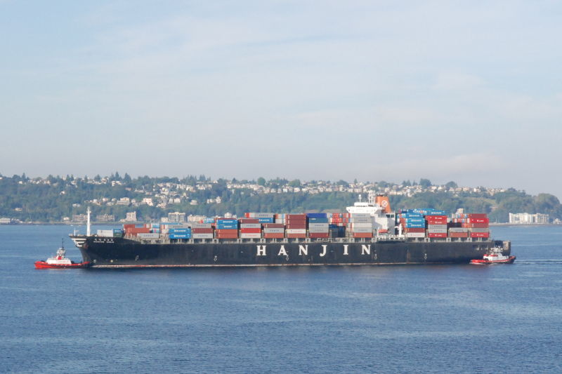
Think of the scientists who, over many years, have been, and still are, taking
billions of measurements on the stormy, windy, and undulating high seas.
 |
Fig. 3 Limit 25 rows
|
That
over one hundred seventy three million measurements I am working with is a tiny fraction of the whole (it will double, or more as I download more zones and add the v2 salinity).
BTW, you may be wondering what the "raw1000_v1, raw3000_v1, raw5000_v1, and raw7000_v1" names are about (the 'v1' means WOD variable 1, which is temperature; 'v2' is salinity which I have not gotten to yet, but I have them substantially downloaded and ready for their SQL tables).
Those who have viewed
the WOD database will note that there are four basic zone sections (
1000,
3000,
5000, and
7000).
From a programing perspective, they are defined by the first digit (1,3,5,7).
Each of those has nine subsections (0 - 8), which again, from a programming perspective, are defined by the second digit (1
000, 3
100, 5
500, and 7
800, etc.).
Those in turn have eighteen sub-subsections (10
00-10
17), which are defined by the last two digits of a zone's number (incidentally the zone number tells us its latitude and longitude boundaries too).
Anyway, as shown in
Fig. 2, the zone numbers add up to 648 WOD zones (4 × 9 × 18 = 648).
 |
| Fig. 4 2,007,831 rows |
A software developer has to deal with the original situation as it is, not how they would do it (I like the WOD numbering system).
In this case, a "tree" structure is the way I chose to handle this problem, because there are gaps.
One can't use a 648 element array because the zone numbers are not sequential.
They proceed as 1000-1017 (gap 1018 - 1099), then proceed as 1100-1117 (more gaps on the way to 1817), then the 3000-3017 series begins, (gap 3018 - 3099) 3100-3117 (gaps ...) etc. etc. so the tree structure is an efficient way to code a traverse of the WOD zones (see
Fig. 2).
Notice
Fig. 3 and
Fig. 4 to get a glimpse of what the rows of records look like "in the raw."
The SQL query that produced the list in
Fig. 3 has an SQL "limit 25" clause in it, so it only produced 25 rows.
 |
| Fig. 5 the history table |
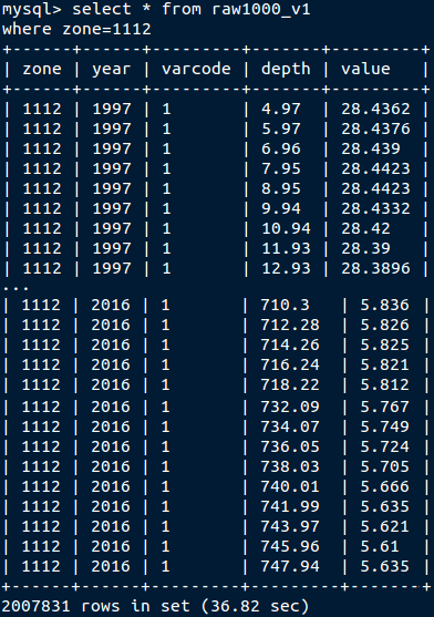
I "let fly" with
Fig. 4 by removing that limit, so it retrieved all rows for that zone.
But, I can't show you all 2,007,831 rows in zone 1112 ... it would fill way too many blog pages.
But you get my drift, there is a lot of data to look at, so I have to tailor results to viable blog post lengths.
Notice the
many different depths in meters (next to last column @
Fig. 4) just so you understand that I also had to deal a blow to
the volume of data involved.
 |
| Fig. 6 Finally, a graph ! |
I did so by using the "0-200", "200-400", "400-600", "600-800", "800-1000", "1000-3000", and ">3000" depth levels ('>' means greater than).
All the many variant depths and values are isolated to, or are averaged (by year) into seven levels, covering the entire water column from the surface to the bottom.
What this all boils down to is depicted in
Fig. 5, which shows the SQL query in the 'history' table (which is what is produced from the '2,007,831 rows' @
Fig. 4) on WOD Zone 1112, after the condensing.
Then, what
you typically are shown is the graph at
Fig. 6.
In this post I have not mentioned the downloading and
slicing of the PI data (my nickname for their file format) because that was covered in the previous post.
Now you know why I was also critical, in the previous post, of the scientist who wanted to
estimate these billions of measurements with a "mathematical model":
With recently improved instrumental accuracy, the change in the heat content of the oceans and the corresponding contribution to the change of the sea level can be determined from in situ measurements of temperature variation with depth. Nevertheless, it would be favourable if the same changes could be evaluated from just the sea surface temperatures because the past record could then be reconstructed and future scenarios explored. Using a single column model we show that the average change in the heat content of the oceans and the corresponding contribution to a global change in the sea level can be evaluated from the past sea surface temperatures.
(
Ocean Science, 6, 179–184, 2010, emphasis added). And that ill-advised misadventure was advocated without even going to ARGO land where the PFL measurements are made by accurate automated submersibles (
ARGO net).
[The WOD "PFL" files are robust: "
Note: WOD includes GTSPP and Argo data, plus more" -
Ocean Profile Data]
The next post in this series is
here, the previous post in this series is
here.