The Evolution of Models - 2

Fig. 1 (click to enlarge)

Today, I am going to be "talking out loud" about the sea level rise (SLR) calculation program, version 1.0 (earlier versions I posted about were betas).

I added a masking class that normalizes the candidate data being used for a particular year's calculation utilizing the track urged by the Potsdam Institute authors in a paper they published in PNAS (Potsdam Institute, cf. PNAS).

By "normalizing" I mean the software logic influences the calculation by utilizing the principle of 2.3 meters of SLR per 1 degree centigrade of increased global temperature as shown in Fig. 1 above, and as discussed in the paper.

The purpose of Fig. 1 is to show the SLR generated by those global temperatures and the time the potential was generated.

The purpose is not to show when that SLR will be actualized in reality.

To the degree that the data is outside that track, it modifies it closer to a track in line with that formula, but only to a degree, and only if directed to do so.

That nudge bends any calculation to the generally accepted history of average global temperatures used by many climate scientists, bloggers, educators, etc. (NOAA).

In other words, if the data presented to the model is suggesting X, but X is either higher or lower than "2.3 meters of SLR per 1 degree centigrade of increased global temperature" it is modified closer to that norm.

The rub in using the Potsdam formula comes when models attempt to implement the delay between the time of temperature rise, and the resulting impact on ice melt caused SLR.

Traditionally, that delay has been about 40 years for some scenarios, but can vary (Time Keeps on Slippin' Slippin' Slippin' In From The Past).

The Potsdam Institute writes about long delay time frames, so by default I staggered it by 100 years (1880-2014 becomes 1980-2114) in the masking, but that can be modified downward (decreased) by a data setting (as are the other relevant parameters that control the modelling program).

Those parameters can be in either an SQL or a flat-file database.

Anyway, I eventually want to have several masks based on formulas using observed, measured, and known values for those instances where the model is being used in scenarios requiring as little speculation as possible.

That is because the model, being data driven, will generate any scenario, real or fanciful, that the user wishes to generate data and graphs for.

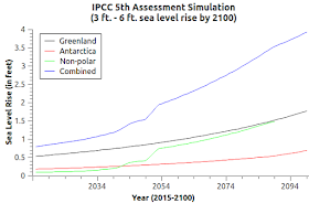
For example, Fig. 2 is generated by a data set to simulate the IPCC 3 ft. to 6 ft. SLR by about 2100.

Fig. 2 (click to enlarge)

Any scenario can be modelled.

The way I do it is to write a "mySQL" script file that creates an SQL table in a mySQL database, then populates the table with data for the desired scenario.

For instance, Fig. 3 shows about a 21 ft. SLR by 2100 using a different dataset.

That is, it was generated using a different SQL script file in order to generate a different database table.

Fig. 3 (click to enlarge)

One can create as many of those files as desired, and use them any time, which beats continual data entry any time a different scenario is desired.

As our knowledge improves those files can improve and therefore the model will generate a better picture of prospective SLR in future years.

One can only wonder as to why this has not been basic protocol and practice, but one thing, fear of reality comes to mind as a reoccurring phenomenon.

The model, as I have written before, is based on four zones (coastal, inland 1, inland 2, and no-melt) in each area where relevant ice sheets exist (non-polar glaciers, ice caps; Greenland; and Antarctica).

The accuracy of the model's work depends on the accuracy of the values associated and attributed to each zone.

Thus, to the degree that the size of the zone (stored in the data that the model uses) is inaccurate, is the degree to which the projections will be inaccurate.

So, keeping a close eye on scientific research and findings on the ice volume in the zones in Antarctica and Greenland, then updating the database accordingly, will improve the results.

Likewise, it is essential to assign accurate acceleration rates to each zone in order to enhance accuracy.

It is all about accurate data.

The next post in this series is here, the previous post in this series is here.

---

---